Several months ago I made a game based on a soft-body physics engine for Ludum Dare 53. It looks like this:
I made a detailed blog post on how to implement such a physics engine, and one crucial part of this engine was shape matching: given initial positions of some points, and their final positions, compute the rotation from the former to the latter such that the rotated initial positions best approximate the given final positions.
In 2D, a rotation can be specified by just an angle, and we were able to derive an very neat explicit exact formula for this angle:
\[ \theta = -\operatorname{atan2}\left(\sum r_i\times q_i, \sum r_i \cdot q_i\right) \]I didn't talk about solving this problem in 3D, though, thinking that I'll postpone this until I actually need to implement a 3D soft-body physics engine.
However, this problem emerged in a place where I didn't expect it to.
Contents
Simulating cloth
I spent the December of 2023 trying out WebGPU – a new graphics API which seemed more modern and less weird than OpenGL, and yet less complex and low-level than Vulkan. I made a nice demo project that renders the Sponza scene with a few fun additions:

In particular, this project features cloth simulation:
It is done by taking the original mesh of a cloth object, and treating all mesh edges as undamped springs. Then some velocity diffusion is added to make the cloth less jittery, and some velocity damping to simulate air friction.
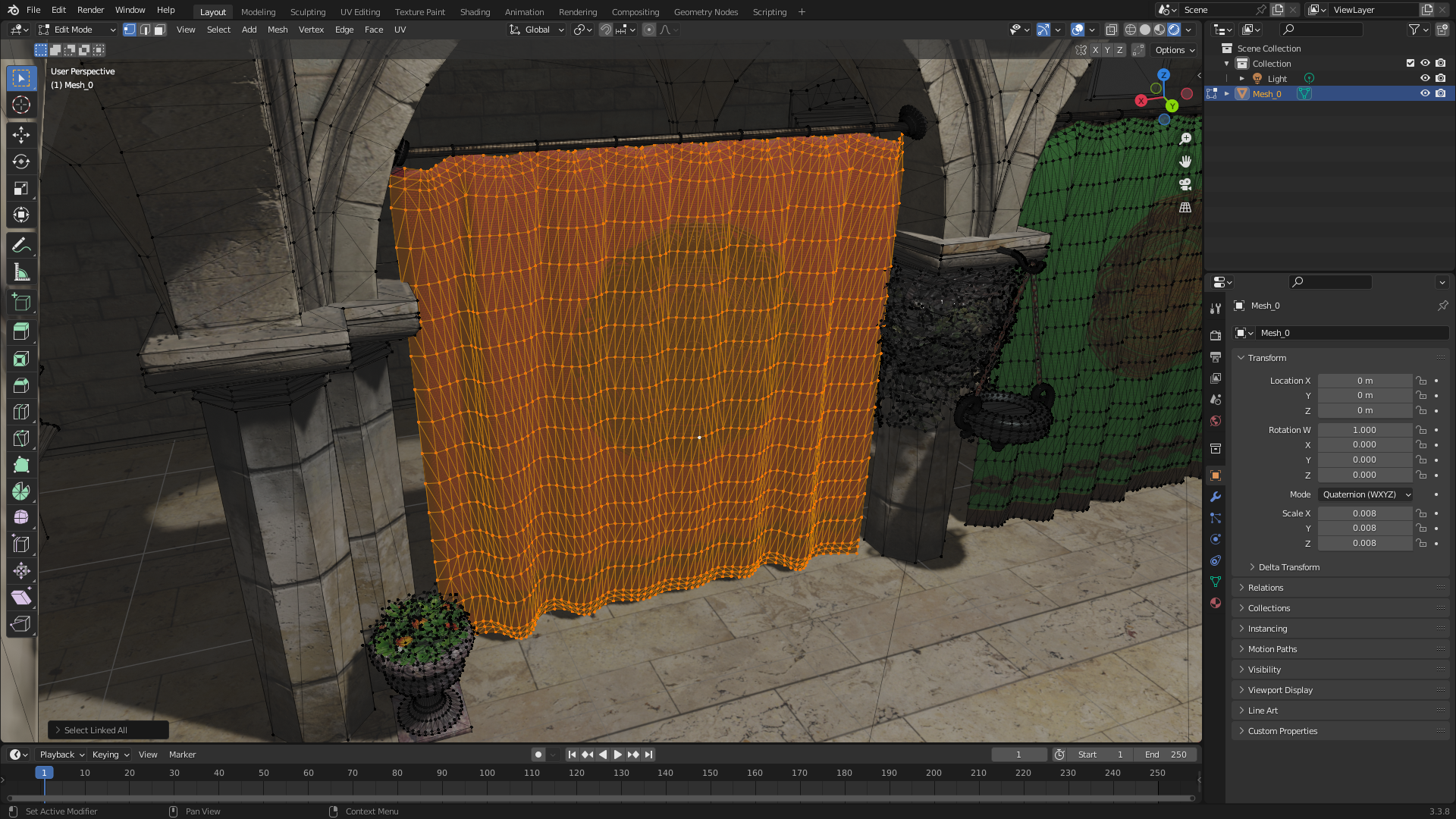
There's a catch, though. The vertices of the mesh don't just have positions, they also have normal and tangent vectors needed to properly compute lighting on the cloth (in particular, tangents are used in normal mapping). If we displace the positions of the vertices, their normals and tangents should also change!
Now, of course there are ways to reconstruct these vectors. The normal can be approximated as the weighted average of all normals for the triangles containing the vertex. The tangent vector can be approximated from the UV coordinates of the nearby vertices. In fact, some implementations of normal/bump mapping don't use tangents at all, but rely on some pixel-local UV trickery.
However, there is also a stupidly generic way to solve this problem, which is to realize that it is an instance of 3D shape matching! See, we have initial vertex positions, we have final vertex positions (after doing the cloth simulation), and we want to compute the rotation that moves the former to the latter. Then, we simply apply this same rotation to normal and tangent vectors!
This should be done in the local neighbourhood of each mesh vertex, i.e. treat your current vertex as the world origin, and take its neighbouring vertices as the data for the shape matching problem.
Before we dive into how this can be done in 3D, let's revisit the 2D case.
2D shape matching with complex numbers
Let's formalize our problem first. We have the initial vectors \( a_k \) (think of them as vectors from the current vertex to its neighbouring vertices) and the final vectors \( b_k \) (again, vectors from the vertex to its neighbours, but after the simulation altered the vertex positions), and we want to find a rotation \( R \) which minimizes the error
\[ E = \sum \| Ra_k - b_k \| ^2 \]By expanding the squared length, we get
\[ \sum (Ra_k - b_k)\cdot (Ra_k - b_k) = \sum (Ra_k)\cdot(Ra_k) - 2 Ra_k\cdot b_k + b_k\cdot b_k = \] \[= \sum \|a_k\|^2 - 2 Ra_k\cdot b_k + \|b_k\|^2 \]We've used that \( \|Ra_k\| = \|a_k\| \), since \( R \) is a rotation. Now, \( \|a_k\|^2 \) and \( \|b_k\|^2 \) don't depend on \( R \), so we can throw them away, and we're left with minimizing
\[ \sum - 2 Ra_k\cdot b_k \]or, changing signs and removing the useless factor of \( 2 \), maximing
\[ \sum Ra_k\cdot b_k \]This has a nice geometric interpretation: the dot product of \( Ra_k \) and \( b_k \) is largest when they point in the same direction, so we need to find a rotation \( R \) such that the vector \( Ra_k \) points in the direction of \( b_k \) as much as possible, which sounds like exactly what we're trying to do!
This was all not specific to 2D, and works in any dimension. Now let's turn to 2D, where any rotation is always of the form
\[ \begin{pmatrix} \cos \theta & -\sin \theta \\ \sin \theta & \cos \theta \end{pmatrix} \]and we can analytically find the angle \( \theta \) that minimizes the error \( E \). However, we can use a different approach: complex numbers!
By treating our 2D vectors \( a_k \) and \( b_k \) as complex numbers, we can represent a rotation by angle \( \theta \) as complex multiplication by \( e^{i\theta} \). What's more, we can express the dot product by complex multiplication, conjugation, and taking the real part: \( a \cdot b = \operatorname{Re}(a\bar b) \). With this in mind, we can rewrite the error \( E \) as
\[ E = \sum \operatorname{Re}\left(e^{i\theta}a_k\bar b_k\right) = \operatorname{Re}\left(e^{i\theta}\sum a_k\bar b_k\right) \]Now, \( z = \sum a_k\bar b_k \) is just some complex number, and multiplication by \( e^{i\theta} \) rotates it by \( \theta \) radians counterclockwise. Maximizing the real part \( \operatorname{Re} \) of the product \( e^{i\theta}z \) means we need this product to point to the right from the origin in the complex plane, i.e. we want it to be a positive real number. In order to do this, we need to find the angle that \( z \) forms with the positive real axis, and take \( \theta \) to be minus that angle (i.e. to rotate backwards). This angle is
\[ \operatorname{atan2}\left(\operatorname{Im}(z), \operatorname{Re}(z)\right) \]so
\[ \theta = -\operatorname{atan2}\left(\operatorname{Im}(z), \operatorname{Re}(z)\right) \]Now all we need is compute the real and imaginary parts of \( z \). For that we need a few fun identities. Have a look at \( a\bar b \):
\[ a\bar b = (a_{real} + ia_{imag})\overline{(b_{real} + ib_{imag})} = (a_{real} + ia_{imag})(b_{real} - ib_{imag}) \] \[ = (a_{real}b_{real} + a_{imag}b_{imag}) + i(a_{real}b_{imag}-a_{imag}b_{real}) = \operatorname{dot}(a,b) + i\operatorname{cross}(a,b) \]So, the real part is just the dot product of \( a \) and \( b \), while the imaginary part is the 2D cross product! And the final formula is
\[ \theta = -\operatorname{atan2}\left(\sum a_k \times b_k, \sum a_k\cdot b_k \right) \]exactly as we've shown in the previous post.
Does it help us with the 3D case, though? No, not really. This particular calculation doesn't easily generalize to 3D and quaternions. We need a different perspective.
2D shape matching with eigenvalues
Let's return to our original problem formulation, but still in complex numbers. I'll define \( r = e^{i\theta/2} \), and notice that our rotation is \( r^2 \), not just \( r \). This will make sense soon. Also keep in mind that \( r \) is a unit vector, i.e. it has length 1. We want to minimize
\[ \sum \|r^2a_k - b_k\|^2 \]Now, since in complex numbers the length of a product is the product of lengths, we can safely multiply be the length of \( r^{-1} = \bar r \), because it is also 1:
\[ \sum \|r^2a_k - b_k\|^2 = \sum \|r^2a_k - b_k\|^2 \|r^{-1}\|^2 = \sum \|ra_k - \bar r b_k\|^2 \]This is cool, because now the \( ra_k - \bar r b_k \) part is a linear function of \( r \)! Let's call this linear transformation \( S_k \). It is a real-valued matrix acting on complex numbers as 2D vectors, so it is a \( 2\times 2 \) matrix. We don't need its explicit form just yet.
Now we can forget that these were complex numbers. All we have is a 2D unit vector \( r \), and we want to minimize
\[ \sum \|S_k r\|^2 \]The dot product of two column vectors can be written in matrix form using the transpose operation as \( c \cdot d = c^{T} d \). A squared length is the same as dot product with itself, so
\[ \sum \|S_k r\|^2 = \sum (S_k r)^{T} (S_k r) = \sum r^{T} (S_k ^T S_k) r = r^T \left(\sum S_k^TS_k\right)r = r^T B r \]where
\[ B = \sum S_k^T S_k \]All \( S_k^TS_k \) are symmetric positive-semidefinite \( 2\times 2 \) matrices, and so is \( B \). The expression \( r^T B r \) is a quadratic form, and we need to minimize it.
This is where we're golden: it is a well-known theorem that the minimum of a quadratic form applied to unit vectors is the smallest eigenvalue of the matrix \( B \), and the actual minimizing vector is the corresponding eigenvector! So, all we need to do is compute this \( 2\times 2 \) matrix and slap an eigenvector algorithm on top of it!
This sure does sound much more complicated than an explicit formula, so why even bother? Well, because this is what actually generalizes to 3D.
3D shape matching with quaternions and eigenvalues
In 3D, our task is exactly the same: minimize
\[ E = \sum \| Ra_k - b_k \|^2 \]where \( R \) is a 3D rotation operator. Of course, we want to express this rotation as a unit quaternion \( q \), so that \( Ra = qaq^{-1} \). This gives
\[ E = \sum \| qa_kq^{-1} - b_k \|^2 \]We employ the same trick: since the length of a product is equal to the product of lengths of quaternions, we can multiply by the squared length of \( q \) on the right (quaternion multiplication isn't commutative, so it matters on which side we multiply):
\[ \sum \| qa_kq^{-1} - b_k \|^2 = \sum \| qa_kq^{-1} - b_k \|^2 \|q\|^2 = \sum \| qa_k - b_kq \|^2 \]Now, this \( qa_k-b_kq \) is again a linear operator \( S_k \) applied to \( q \), only this time it is a \( 4\times 4 \) real matrix, because quaternions are 4-dimensional. After that, we forget about quaternions and return to matrices:
\[ \sum \| qa_k - b_kq \|^2 = \sum \|S_k q\|^2 = q^T \left(\sum S_k^T S_k\right) q = q^T B q\]Explicitly computing \( B \) is a bit tiresome but still straightforward (just write in coordinates what \( qa_k - b_kq \) does to the coordinates of \( q \)). And again we have a quadratic form, and we need to find the eigenvector corresponding to the smallest eigenvalue! This time the matrix is \( 4\times 4 \) – not too bad, but an explicit formula would involve solving a generic quartic equation, which is nuts.
In fact, computing eigenvalues is pretty much equivalent to computing roots of polynomials (see the companion matrix), so there is no general eigenvalue algorithm for matrices of arbitrary size that just uses an explicit formula. Instead, all such algorithms are iterative, and converge to the solution as the number of iterations grows. See here for a list of such algorithms.
The code
I didn't want to do anything computationally expensive here (after all, this needs to be done for each of the vertices of the cloth mesh, on each rendering frame), so I pretended I know nothing about matrices and just regarded \( q^T B q \) as some arbitrary function, and minimized it with a single iteration of gradient descent on each frame. Since these rotations don't change too much from frame to frame, I can use the rotation computed on the previous frame as a good initial guess.
I was using WGSL in my project (the shading language that comes with WebGPU). To construct the matrix \( B \), I needed a few helping functions that essentially encode the quaternion multiplication formula:
// The matrix of the linear operator (q -> q * a)
fn rightMultMatrix(a : vec4f) -> mat4x4f {
    return mat4x4f(
        vec4f( a.w, -a.z,  a.y, -a.x),
        vec4f( a.z,  a.w, -a.x, -a.y),
        vec4f(-a.y,  a.x,  a.w, -a.z),
        vec4f( a.x,  a.y,  a.z,  a.w),
    );
}

// The matrix of the linear operator (q -> b * q)
fn leftMultMatrix(b : vec4f) -> mat4x4f {
    return mat4x4f(
        vec4f( b.w,  b.z, -b.y, -b.x),
        vec4f(-b.z,  b.w,  b.x, -b.y),
        vec4f( b.y, -b.x,  b.w, -b.z),
        vec4f( b.x,  b.y,  b.z,  b.w),
    );
}
Then, to compute the matrix \( B \), we just need to iterate over the neighbouring vertices and sum the corresponding terms:
var errorMatrix = mat4x4f(vec4f(0.0), vec4f(0.0), vec4f(0.0), vec4f(0.0));

let currentPosition = clothVertices[id.x].newPosition;

for each edge {
    let initialDelta = ...; // a_k
    let currentDelta = ...; // b_k

    let m = rightMultMatrix(vec4f(initialDelta, 0.0))
          - leftMultMatrix(vec4f(currentDelta, 0.0));

    errorMatrix += transpose(m) * m;
}(for each edge is, of course, pseudo-code)
And finally I do a single iteration of gradient descent with a step size picked by hand, followed with a projection onto the space of unit vectors (i.e. a normalize call). Note that the gradient of \( q^T B q \) is just \( 2 q^T B \).
let rotationGrad = 2.0 * rotation * errorMatrix;
rotation = normalize(rotation - rotationGrad * 0.25);
The actual compute shader code for this thing is here.
The result
Now, does this thing actually work? Yep, it does! I confirmed this by rendering the normals as colors, and visually confirming that they point in the direction that they should.
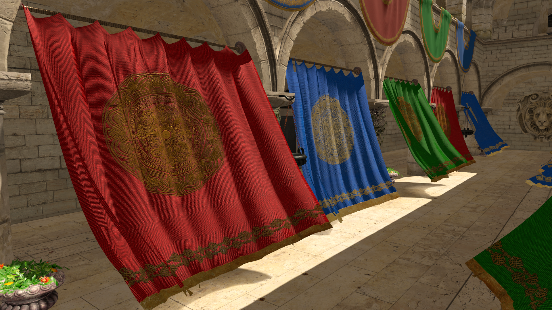
Another way to validate this solution is to look at how it affects shading. Before applying this reconstruction algorithm, the cloth was shaded always the same as it would be in the initial mesh, without cloth simulation applied:
While after using this algorithm, the cloth properly reacts to the changes:
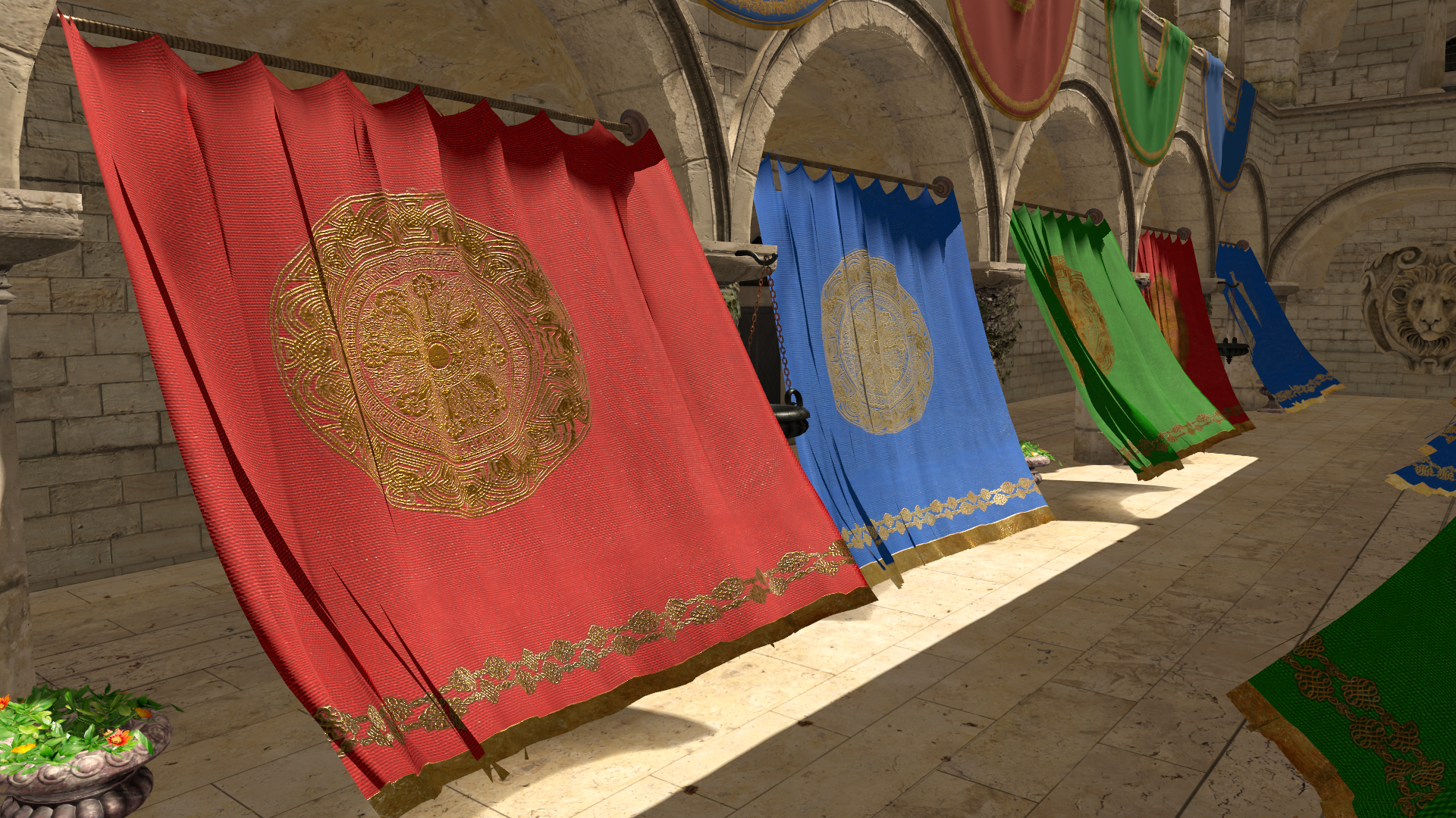
And this is how it looks in motion:
The end
So, there's that! Honestly, if I were to make a 3D soft body physics engine, I'd probably do a QR algorithm instead of a gradient descent, or maybe the Jacobi eigenvalue iteration which works specifically for symmetric matrices. It shouldn't be too hard for a \( 4\times 4 \) matrix. I hope to do that some day, maybe on another game jam :)
And, as always, thanks for reading!