Recently (well, a few months ago), I was adding support for animated models in my traffic simulation game. Specifically, I wanted to animate windmills:
Of course, this is extremely easy to hard-code (have two objects, one static and one rotating). However, I was planning to add more animations later, so I decided to implement a proper solution.
Previously I used a crappy ad-hoc binary format for models and animations, but I've recently switched to glTF for a number of reasons:
- It is easy to parse: JSON metadata + raw binary vertex data
- It is easy to render: models are stored in a format that maps directly to graphics API's
- It is compact enough (the heavy stuff – vertex data – is stored in binary)
- It is widespread and extensible
- It supports skeletal animations
Using glTF models means it is easy for others to extend the game (to author mods, for example).
Unfortunately, finding a good resource on skeletal animation with glTF specifically seemed impossible. All tutorials cover some older formats, while the glTF specification, being mostly quite verbose and precise, is unusually terse when it comes to the interpretation of the animation data. I guess it should be obvious to experts, but I'm not one of them, and if you're not either – this is an article for you :)
Btw, I ended up reverse-engineering Sascha Willems's animation code in his Vulkan + glTF example renderer to figure out how to do this properly.
Contents
Skeletal animation
If you already know what skeletal animation is, you can safely skip this section :)
Skeletal animation is by far the most popular method for animating 3D models. It is pretty simple conceptually: instead of animating the actual model, you animate a virtual highly simplified skeleton of the model, and the model itself is glued to this skeleton, like meat to the bones. Here's how it looks, roughly:
Here's how the vertices of the model are glued to different bones (red is a lot of glue, blue is no glue):
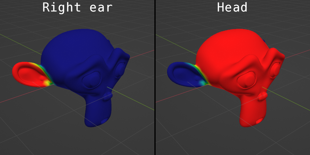
Typically, each mesh vertex is glued to several bones with different weights to provide smoother animations, and the resulting transformation of the vertex is interpolated between these bones. If gluing each vertex to just a single bone, the transitions between different parts of the model (e.g. typically human shoulders, elbows and knees) will experience unpleasant artifacts when animated:
Another crucial part of this method is that it is hierarchical: the bones form a tree, with child bones inheriting their parent's transformation. In this example model, the two ear bones are children to the head bone, which is the root of the skeleton. Only the head bone is explicitly rotated up and down; the ears inherit this rotation from the head bone.
This is for the same reason why most game engines use object hierarchies. When you have a mosquito on a helmet on a man in a car on a moving carrier ship, it's quite tiresome and error-prone to define the movement of all these objects separately. Instead, one would define the ship's movement, and specify that the objects form a hierarchy, with the children inheriting the parent's movement. The mosquito would be a child of the helmet, the helmet – a child of the man, and so on.
Likewise, it is much easier to specify that the human's shoulder is rotating (and the whole arm rotating as per being a child of the shoulder), instead of computing the proper rotations for each of the arm's bone.
Pros'n'cons
Compared to the alternative method – morph-target animation, which stores all vertices' positions for each animation frame (and is also supported by glTF), – it has some advantages:
- It requires less storage – the skeleton is much smaller than the model
- Less data streaming is required per frame (only the bones, as opposed to the whole mesh, – although there are ways to store the whole animation on the GPU)
- It is (arguably) easier to work with for an artist
- It decouples animation from a specific model – you can have the same walking animation applied to many different models with different numbers of vertices
- It is much easier to integrate into procedural animation – say, you want to constrain a character's foot not to get through terrain; with skeletal animation, you only need to add constraints to a few bones
It has a couple of downsides, though:
- You need to properly parse/decode the animation format you're using (this is harder than it sounds)
- You need to compute the transform for each bone for each animated model, which can be costly and also tricky (though one could do that using compute shaders)
- You need to somehow transfer the bones data to the GPU, which are not a vertex attribute and might not fit into uniforms
- You need to apply the bone transforms in the vertex shader, making this shader something like 4x slower than usual (still much cheaper than the typical fragment shader, though)
It isn't as bad as it sounds, though. Let's dive into how you'd implement that, bottom-up.
Bone transforms
So, we need to transform our mesh vertices somehow, on the fly. Each bone defines a certain transformation, – typically composed of scaling, rotation and translation. Even if you don't need scaling and translation, and your bones only rotate (which is reasonable for many realistic models – try moving your shoulder half a meter out of the shoulder socket!), the rotation can still happen around different centers of rotation (e.g. when an arm rotates around a shoulder, the hand also rotates around the shoulder and not around the hand bone origin), meaning you still need translations anyway.
The most general way to support all this is to simply store a \(3\times 4\) affine transformation matrix per each bone. This transformation is usually the composition of scaling, rotation and translation (applied in that order), expressed as a matrix in homogeneous coordinates (this is a mathematical trick to express translations as matrices, among other things).
Instead of using a matrix (which is 12 floats), we could separately store a translation vector (3 floats), a rotation quaternion (4 floats), and possibly a uniform (1 float) or non-uniform (3 floats) scaling vector, giving 7, 8 or 10 floats in total. However, as we'll see later, it is easier to pass these transformations to a shader if the total number of components is a multiple of 4. So, my favourite options are translation + rotation + uniform scale (8 floats) or a full-fledged matrix (12 floats).
In any case, these transformations should already account for the parent's transformations as well (we'll do this a bit later). Let's call them global transforms, instead of local transforms which don't account for the parents. So, we have a recursive formula like this:
\[ \text{globalTransform(bone)} = \text{globalTransform(parent)} \cdot \text{localTransform(bone)} \]If a bone doesn't have a parent, its globalTransform coincides with the localTransform. We'll talk about where these localTransforms come from later in the article.
Composing transforms
By the way, the above equation might be a bit misleading. If we store transforms as matrices, how do we multiply two \(3\times 4\) matrices? This is against the rules of matrix multiplication! If we store them as (translation,rotation,scale) triplets, how do we compose them?
In the matrix case, the usage of \(3\times 4\) matrices is actually an optimization. What we really need are \(4\times 4\) matrices, which are easy to multiply. It just so happens that affine transformations are always of the form
\[ \begin{pmatrix} a_{11} & a_{12} & a_{13} & t_{1} \\ a_{21} & a_{22} & a_{23} & t_{2} \\ a_{31} & a_{32} & a_{33} & t_{3} \\ 0 & 0 & 0 & 1 \end{pmatrix} \]So, there is no point in actually storing the 4-th row, but we need to restore it when doing computations. In fact, the invertible affine transformations are a subgroup of the group of all invertible matrices.
The recipe for matrices is as follows: append a \( \begin{pmatrix}0 & 0 & 0 & 1\end{pmatrix} \) row, multiply the resulting \(4\times 4\) matrices, and discard the last row of the result, which will also be \( \begin{pmatrix}0 & 0 & 0 & 1\end{pmatrix} \). There are ways to do this more efficiently by explicitly applying the left matrix to the columns of the right matrix, but the general formula is still the same.
Now, what's with storing the transforms explicitly as translations, rotations, and scalings, how do we multiply them? Well, there is just a formula for that! Let's denote our transformations as \( (T,R,S) \) – Translation vector, Rotation operator and Scaling factor. The effect of this transformation on a point \(p\) is \( (T,R,S)\cdot p = T + R\cdot(S\cdot p) \). Let's see what happens if we combine two such transformations:
\[\color{blue}{(T_2,R_2,S_2)}\cdot\color{red}{(T_1,R_1,S_1)}\cdot p = \color{blue}{(T_2,R_2,S_2)}\cdot(\color{red}{T_1} + \color{red}{R_1S_1}p) = \\ = \color{blue}{T_2}+\color{blue}{R_2S_2}(\color{red}{T_1}+\color{red}{R_1S_1}p) = (\color{blue}{T_2}+\color{blue}{R_2S_2}\color{red}{T_1}) + (\color{blue}{R_2}\color{red}{R_1})(\color{blue}{S_2}\color{red}{S_1})p\]I've used the fact that uniform scaling commutes with rotations. In fact, it commutes with anything!
So, the formula for multiplying two transformations in this form is
\[ \color{blue}{(T_2,R_2,S_2)}\cdot\color{red}{(T_1,R_1,S_1)} = (\color{blue}{T_2}+\color{blue}{R_2S_2}\color{red}{T_1}, \color{blue}{R_2}\color{red}{R_1}, \color{blue}{S_2}\color{red}{S_1}) \]Note that \(R\) is the rotation operator (i.e. rotation matrix), not the rotation quaternion. For a rotation quaternion \(Q\), the composition of rotations doesn't change, but the way it acts on a vector does change:
\[ R\cdot p = Q\cdot p \cdot Q^{-1} \] \[ (T,Q,S)\cdot p = T + S\cdot(Q\cdot p \cdot Q^{-1}) \] \[ \color{blue}{(T_2,Q_2,S_2)}\cdot\color{red}{(T_1,Q_1,S_1)} = (\color{blue}{T_2}+\color{blue}{S_2Q_2}\color{red}{T_1}\color{blue}{Q_2^{-1}}, \color{blue}{Q_2}\color{red}{Q_1}, \color{blue}{S_2}\color{red}{S_1}) \]Also note that this trick doesn't work for non-uniform scaling: essentially, if \(R\) is a rotation and \(S\) is a non-uniform scaling, there is no way to express the product \( S\cdot R \) as something like \( R'\cdot S' \) for some other rotation \(R'\) and non-uniform scaling \(S'\). In this case, it's simpler to just use matrices instead.
The vertex shader
That was quite a mouthful of explanations! Let's get to some real code, specifically the vertex shader. I'll use GLSL, but the specific language or graphics API doesn't matter much here.
Say we've passed the per-bone global transforms into the shader somehow (we'll talk about it in a minute). We also need some way to tell which vertex is connected to which bone and with what weight. This is typically done with two extra vertex attributes: one for the bone ID's and one for the bone weights. Usually you don't need more than 256 bones per model, and you also don't need that much precision for the weights, so one can use integer uint8 attribute for the ID's and normalized uint8 attribute for the weights. Since the attributes are at most 4-dimensional in most graphics APIs, we usually only allow a vertex to be glued to 4 bones or less. If, for example, a bone is glued to only 2 bones, we just append two random bone ID's with zero weights and call it a day.
Enough talking:
// somewhere: mat4x3 globalBoneTransform[]

uniform mat4 uModelViewProjection;

layout (location = 0) in  vec3 vPosition;
// ...other attributes...
layout (location = 4) in ivec4 vBoneIDs;
layout (location = 5) in  vec4 vWeights;

void main() {
    vec3 position = vec3(0.0);
    for (int i = 0; i < 4; ++i) {
        mat4x3 boneTransform = globalBoneTransform[vBoneIDs[i]];
        position += vWeights[i] * (boneTransform * vec4(vPosition, 1.0));
    }

    gl_Position = uModelViewProjection * vec4(position, 1.0);
}
In GLSL, for a vector v, v[0] is the same as v.x, v[1] is v.y and so on.
What we do here is
- Iterate over the 4 bones the vertex is attached to
- Read the ID of the bone
vBoneIDs[i]and fetch it's global transform - Apply the global transform to the vertex position in homogeneous coordinates
vec4(vPosition, 1.0) - Add the weighted result to the resulting vertex
position - Apply the usual
MVPmatrix to the result
This whole process is also called skinning, or a bit more specifically linear blend skinning, because we're linearly interpolating between the result of skinning by several bones.
In GLSL matNxM means N columns and M rows, so mat4x3 is actually a 3x4 matrix. I love standards.
If you're not sure that your weights sum up to 1, we can also divide by their sum in the end (although you better be sure they sum up to 1!):
position /= dot(vWeights, vec4(1.0));If the sum of weigts isn't equal to 1, you'll get distortions. Essentially, your vertex will get closer to or further from the model origin (depending on whether the sum is < 1 or > 1). This is related to the perspective projection and also to the fact that affine transformations don't form a linear space, but they do form an affine space.
If we also have normals, those need to be transformed as well. The only difference is that position is a point, while a normal is a vector, so it has a different representation in homogeneous coordinates (we append 0 as the w coordinate instead of appending 1). We might also want to normalize it afterwards, to account for scaling:
// somewhere: mat4x3 globalBoneTransform[]

uniform mat4 uModelViewProjection;

layout (location = 0) in  vec3 vPosition;
layout (location = 1) in  vec3 vNormal;
// ...other attributes...
layout (location = 4) in ivec4 vBoneIDs;
layout (location = 5) in  vec4 vWeights;

vec3 applyBoneTransform(vec4 p) {
    vec3 result = vec3(0.0);
    for (int i = 0; i < 4; ++i) {
        mat4x3 boneTransform = globalBoneTransform[vBoneIDs[i]];
        result += vWeights[i] * (boneTransform * p);
    }
    return result;
}

void main() {
    vec3 position = applyBoneTransform(vec4(vPosition, 1.0));
    vec3 normal = normalize(applyBoneTransform(vec4(vNormal, 0.0)));

    // ...
}
Note that if you're using non-uniform scaling, or you want to do eye-space lighting, things get a bit more complicated.
Passing the transforms to the shader
I'm mostly using OpenGL 3.3 for my graphics stuff, so the details of this section are OpenGL-specific, bit I believe the general concepts apply to any graphics API.
Most skeletal animation tutorials suggest using uniform arrays for the bone transforms. This is a simple working approach, but it can be a bit problematic:
- OpenGL has a limit on the number of uniforms. OpenGL 3.0 guarantees at least 1024 components, meaning single elements of our matrices, loosely speaking. So for
mat4x3, which takes 12 components, we're bound by having \( 1024/12 \approx 85 \) bones per model. This is already quite a lot, so it might actually be enough. Though, a lot of the uniforms are already used for other stuff (matrices, textures, etc), so we usually have less free uniforms. In reality, we usually have from 4096 to 16384 components. - We'll have to update the uniform array per each animated model, meaning a lot of OpenGL calls & no instancing.
The problem can be somewhat fixed by using uniform buffers:
- By spefication, they have more memory available, but still not that much – typically 64 KB for a buffer.
- We don't need to upload all the bone transforms to uniforms, instead we can upload all the transforms for all model to the buffer all in one go. We still have to call
glBindBufferRangefor each model to speficy where this model's bone data is, so, no instancing.
If you're using OpenGL 4.3 or higher, you can simply store all the transforms in a shader storage buffer object, which have basically unlimited size. Otherwise, you can use buffer textures, which are a way of accessing an arbitrary data buffer pretending it to be a 1D texture. A buffer texture doesn't store anything itself, it only references an existing buffer. It works like this:
- We create a usual OpenGL
GL_ARRAY_BUFFERand fill it with all models' bone transforms each frame, stored as e.g. row-wise matrices (12 floats) or TRS triplets with uniform scaling (8 floats) - We create a
GL_BUFFER_TEXTUREand callglTexBuffer(GL_BUFFER_TEXTURE, GL_RGBA32F, bufferID);–RGBA32Fis the pixel format of this texture, i.e. 4 floats (12 bytes) per pixel (so we need 3 pixels per matrix or 2 pixels per TRS triplet) - We attach the texture to a
samplerBufferuniform in the shader - We read the corresponding pixels in the shader with
texelFetchand convert them to bone transforms
With instanced rendering, a shader for this might look like this:
uniform samplerBuffer uBoneTransformTexture;
uniform int uBoneCount;

mat4x3 getBoneTransform(int instanceID, int boneID) {
    int offset = (instanceID * uBoneCount + boneID) * 3;
    mat3x4 result;
    result[0] = texelFetch(uBoneTransformTexture, offset + 0);
    result[1] = texelFetch(uBoneTransformTexture, offset + 1);
    result[2] = texelFetch(uBoneTransformTexture, offset + 2);
    return transpose(result);
}
Note that we assemble the matrix as a 4x3 matrix (called mat3x4 in GLSL), but reading the rows from the texture and writing it to the columns of the matrix, and then transposing it, switching rows and columns. This is simply because GLSL uses column-major matrices.
Phew
Let's recap a little:
- To animate a model, we attach each vertex to at most 4 bones of a virtual skeleton, with 4 different weights
- Each bone defines a global transform that needs to be applied to the vertices
- For each vertex, we apply the transforms of the 4 bones it is attached to, and average the result using weights
- We store the transforms as TRS triplets or as 3x4 affine transform matrices
- We store the transforms in uniform arrays, uniform buffers, buffer textures, or shader storage buffers
What we're left with is where do those global transforms come from?
Global transforms
Well, actually, we already know where the global transforms come from: they're computed from local transforms:
\[ \text{globalTransform(bone)} = \text{globalTransform(parent)} \cdot \text{localTransform(bone)} \]A naive approach for computing this would be something like a recursive function that computes all transforms:
mat4 globalTransform(int boneID) {
    if (int parentID = parent[boneID]; parentID != -1)
        return globalTransform(parentID) * localTransform[boneID];
    else
        return localTransform[boneID];
}
or the same thing, but with manual unrolling of the tail recursion:
for (int boneID = 0; boneID < nodeCount; ++boneID) {
    globalTransform[boneID] = identityTransform();
    int current = boneID;
    while (current != -1) {
        globalTransform[boneID] = localTransform[current] * globalTransform[boneID];
        current = nodeParent[current];
    }
}
Both these methods are fine, but they compute way more matrix multiplications than necessary. Remember, we're supposed to do this on every frame, for every animated model!
A better way to compute global transforms is to do it from parents to children: if the parent's global transform is already computed, all we need to do is one matrix multiplication per bone.
// ... somehow make sure parent transform is already computed
if (int parentID = parent[boneID]; parentID != -1)
    globalTransform[boneID] = globalTransform[parentID] * localTransform[boneID];
else
    globalTransform[boneID] = localTransform[boneID];
To ensure that parent computations go before children, you'd need some DFS over the bone tree to properly order the bones. An arguably simpler solution is to compute the topological sort of the bone tree (an enumeration of bones such that parents go before children) in advance and use it every frame. (Btw, computing the toposort boils down to DFS anyway.) An even simpler solution is to ensure that the bone ID's effectively are a topological sorting, i.e. that parent[boneID] < boneID always holds. This can be done by reordering the bones (and mesh vertex attributes!) at load time, or by requiring the artists to order their bones this way :) Uhm, their models' bones, that is.
In the latter case, the implementation is the simplest (and the fastest):
for (int boneID = 0; boneID < nodeCount; ++boneID) {
    if (int parentID = parent[boneID]; parentID != -1)
        globalTransform[boneID] = globalTransform[parentID] * localTransform[boneID];
    else
        globalTransform[boneID] = localTransform[boneID];
}
But where do the local transforms come from?
Local transforms
This is where things get a bit quirky (as if they weren't already). You see, it is usually convenient to specify local bone transformations in some special coordinate system instead of the world coordinates. If I rotate my arm, it would make sense that the origin of the local coordinate system is at the center of rotation, and not somewhere at my feet, so that I don't have to explicitly account for this translation. Also, if I rotate it up and down, as if waving to someone at a distance, I'd really want it to be a rotation around some coordinate axis (maybe, X) in the local space, regardless of how the model is oriented in the model space and the world space.
What I'm saying is that we want a special coordinate system (CS) for each bone, and we want the bone local transformations to be described in terms of this coordinate system.
However, the vertices of the model are in, well, the model's coordinate system (that's the definition of this coordinate system). So, we need a way to transform the vertices into the local coordinate system of the bone first. This is called an inverse bind matrix, probably because it sounds really cool.
Ok, we've transformed the vertices to the local CS of a bone, and applied the animation transform (we'll get to them in a moment) in this local CS. Is that all? Remember that the next thing is to combine this with the transform of the parent bone, which will be in it's own coordinate system! So we need another thing: transform the vertex from the bone local CS to the parent's local CS. This can be done using the inverse bind matrices, by the way: transform the vertex from the bone's local CS back to the model CS, and then transform it to the parent's local CS:
\[ \operatorname{convertToParentCS(node)} = \operatorname{inverseBindMatrix(parent)} \cdot \operatorname{inverseBindMatrix(node)}^{-1} \]We can also think of it as follows: a specific bone transforms vertices to it's local CS, applies animation, then transforms them back; then it's parent transforms the vertices to it's own local CS, applies it's own animation, and transforms them back; and so on.
Actually, we don't actually need this converToParent transform explicitly when working with glTF, but it is useful to think about it nevertheless.
There's one more thing. Sometimes, it is convenient (for the artist, or for the 3D modelling software) to attach the vertices to the bones not in the model's default state, but in some transformed state, called the bind pose. So, we might need another transformation which, for each bone, transforms the vertex to the CS that this bone expects the vertices to be in. I know, it sounds confusing, but bear with me, we won't actually need this transformation :)
Click to see a bear

Blender uses world-space vertex positions as the bind pose. If your model is located 20 units along the X-axis from the origin, it's raw vertex positions will be around X=20, and the inverse bind matrices will compensate for that. This effectively renders animated models exported from Blender impossible to use without animation.
Transform recap
In total, we have the following sequence of transformations applied to a vertex:
- Convert it to the model bind pose
- Transform to bone local CS (inverse bind matrix)
- Apply the actual damn animation (specified in local CS)
- Transform back from bone local CS to model CS
- If the bone has a parent, repeat steps 2-5 for the parent bone
Now, the thing is that each format defines its own ways of specifying these. In fact, some of these transforms may even be absent – it is supposed that they are included in the other transforms.
Let's finally talk about glTF.
glTF 101
glTF is a pretty cool 3D scene authoring format developed by Khronos Group – the folks behind OpenGL, OpenCL, Vulkan, WebGL, and SPIR-V, among other numerous things. I've already said why I think it is a cool format in the beginning of the article, so let's talk a bit more on the details.
Here's the specification for glTF-2.0. It is so good that learning the format can be done by just reading the spec.
A glTF scene is composed of nodes, which are abstract and can mean many things. A node can be a rendered mesh, a camera, a light source, a skeleton bone, or just an aggregate parent for other nodes. Each node has its own affine transformation, which defines its position, rotation and scale with respect to the parent node (or the world origin, if it doesn't have a parent).
glTF describes all binary data via accessors – basically, references to a part of some binary buffer containing an array (potentially with non-zero gaps between elements) with a specified type (like e.g. a contiguous array of 100 vec4's with float32 components starting at byte 6340 in this particular binary file, stuff like that).
If a mesh node uses skeletal animation, it has a list of joints which are ID's of glTF nodes that specify the bones of the skeleton. (Actually, the mesh references a skin, which in turn contains the joints.) These joints form a hierarchy – they are still glTF nodes, so they can have parents and children. Note that there's no armature or skeleton node – just the bone nodes; likewise the animated mesh isn't a child of bone nodes or an armature node, but references them indirectly (although exporting software might add an artificial armature node, e.g. Blender does that, – but it isn't required by glTF).
Each vertex attribute of a mesh (actually, of a mesh primitive) – positions, normals, UV's, etc – is a separate accessor. When a mesh uses skeletal animation, it also has bone ID and weight attributes, which are also some accessors. The actual animation of the bones is also stored in accessors.
Along with the description of a skinned mesh, a glTF file may also contain some actual animations – in essence, instructions on how to change the 3rd transform from the list above.
glTF transforms
Here's how glTF stores all the transforms in the 1-5 list above:
- Model bind pose is supposed to be either already applied to the model, or premultiplied to inverse bind matrices. In other words, simply forget about bind pose for glTF.
- The per-bone inverse bind matrices are specified as yet another accessor – an array of 4x4 matrices (which are required to be affine transformations, so only the first 3 rows are interesting).
- The actual animation can be defined externally (e.g. procedural animation), or stored as keyframe splines for the rotation, translation and scale of each bone. The important thing here is that these are...
- ...combined with the transformation from local CS to the parent's local CS. So, the
convertToParentand the bone animation are combined. - The parents are defined by the node hierarchy, but since we've already applied the
convertToParenttransform, we don't need the parent's inverse bind matrix, so we only repeat steps 3-5 for the parent, if any.
So, when working with glTF, the global transform for a bone looks something like
\[ \operatorname{global(bone)} = \ldots \cdot \operatorname{animation(grand-parent)}\cdot\operatorname{animation(parent)}\cdot \\ \cdot \operatorname{animation(bone)}\cdot\operatorname{invBind(bone)} \]And in code this would be
// assuming parent[boneID] < boneID holds

// somehow compute the per-bone local animations
// (including the bone-CS-to-parent-CS transform)
for (int boneID = 0; boneID < boneCount; ++boneID) {
    transform[boneID] = ???;
}

// combine the transforms with the parent's transforms
for (int boneID = 0; boneID < boneCount; ++boneID) {
    if (int parentID = parent[boneID]; parentID != -1) {
        transform[boneID] = transform[parentID] * transform[boneID];
    }
}

// pre-multiply with inverse bind matrices
for (int boneID = 0; boneID < boneCount; ++boneID) {
    transform[boneID] = transform[boneID] * inverseBind[boneID];
}
This transform[] array is the globalBoneTransform[] array in the vertex shader above.
Not that complicated after all! Just need to figure the right order to multiply a bunch of seemingly random matrices :)
glTF animations
Lastly, let's talk about how to apply animations stored directly in glTF files. They are specified as keyframe splines for the rotation, scale and translation of each bone.
Each individual spline is called a channel. It defines:
- Which node (e.g. a skeleton bone) it is applied to
- Which parameter (rotation, scale or translation) it affects
- An accessor for the keyframe timestamps
- An accessor for the keyframe values (
vec4quaternions for rotation,vec3vectors for scale or translation) - An interpolation method –
STEP,LINEAR, orCUBICSPLINE
For rotations, LINEAR actually means spherical linear.
For CUBICSPLINE interpolation, each keyframe stores not one, but 3 values – the spline value and two tangent vectors.
So, the way we build up the local transform for a bone is:
- Sample the splines for the rotation, translation and scale for this bone at the current moment of time
- Combine them together to form the local transformation matrix
For a translation by vector \( (x,y,z) \) the corresponding matrix is
\[ \begin{pmatrix} 1 & 0 & 0 & x \\ 0 & 1 & 0 & y \\ 0 & 0 & 1 & z \\ 0 & 0 & 0 & 1 \end{pmatrix} \]For a non-uniform scaling vector \( (x,y,z) \) the matrix is
\[ \begin{pmatrix} x & 0 & 0 & 0 \\ 0 & y & 0 & 0 \\ 0 & 0 & z & 0 \\ 0 & 0 & 0 & 1 \end{pmatrix} \]and for a unit rotation quaternion \( (x,y,z,w) \) you can find the matrix in the wiki article – it will be a 3x3 matrix which you put into the top-left corner of a 4x4 matrix, like this:
\[ \begin{pmatrix} 1-2(y^2+z^2) & 2(xy-zw) & 2(xz+yw) & 0 \\ 2(xy+zw) & 1-2(x^2+z^2) & 2(yz-xw) & 0 \\ 2(xz-yw) & 2(yz+xw) & 1-2(x^2+y^2) & 0 \\ 0 & 0 & 0 & 1 \end{pmatrix} \]As we've discissed earlier, these matrices are 4x4, but they are really affine transformations, so the interesting stuff only happens in the first 3 rows.
Sampling animation splines
To address the last bit – efficiently sampling the animation splines – we can gather the spline into a class like this:
template <typename T>
struct animation_spline {

    // ...some methods...

private:
    std::vector<float> timestamps_;
    std::vector<T> values_;
};
Now, an obvious API decision would be to make a method that returns the spline's value at some specific time:
template <typename T>
T value(float time) const {
    assert(!timestamps_.empty());

    if (time <= timestamps_[0])
        return values_[0];

    if (time >= timestamps_[1])
        return values_[1];

    for (int i = 1; i < timestamps_.size(); ++i) {
        if (time <= timestamps_[i]) {
            float t = (time - timestamps_[i - 1]) / (timestamps_[i] - timestamps_[i - 1]);
            return lerp(values_[i], values_[i + 1], t);
        }
    }
}
The lerp call should be changed depending on interpolation type and whether this is rotations or not.
This works, but we can improve it in two ways. First of all, our keyframe timestamps are guaranteed to be sorted, so intead of a linear search we can do a binary search:
template <typename T>
T value(float time) const {
    auto it = std::lower_bound(timestamps_.begin(), timestamps_.end(), time);
    if (it == timestamps_.begin())
        return values_.front();
    if (it == timestamps_.end())
        return values_.back();

    int i = it - timestamps_.begin();

    float t = (time - timestamps_[i - 1]) / (timestamps_[i] - timestamps_[i - 1]);
    return lerp(values_[i - 1], values_[i], t);
}
Secondly, when playing an animation, we always traverse it linearly, from start to end, so we could optimize it further by storing the current keyframe index. This isn't a property of animation inself, though, so let's make another class:
template <typename T>
struct animation_spline {

    // ...

private:
    std::vector<float> timestamps_;
    std::vector<T> values_;

    friend class animation_sampler<T>;
};

template <typename T>
struct animation_sampler {
    animation_spline<T> const & animation;
    int current_index;

    T sample(float time) {
        while (current_index + 1 < animation.timestamps_.size() && time > animation.timestamps_[current_index + 1])
            ++current_index;

        if (current_index + 1 >= animation.timestamps_.size())
            current_index = 0;

        float t = (time - timestamps_[current_index]) / (timestamps_[current_index + 1] - timestamps_[current_index]);
        return lerp(values_[current_index], values_[current_index + 1], t);
    }
};
I didn' test this exact code, but I'm using very similar code in my own projects.
What a journey
I hope you liked the article and learnt at least something new today :)
If I messed up something (which I'm absolutely sure I did), feel free to reach out to me somewhere – I'll be happy to fix anything. And, as always, thanks for reading!