First post of the year. Hooray! This year had a truly terrible start for me.
If you're into rendering, you probably know that most modern photorealistic rendering is based on path tracing, which in turn is based on Monte-Carlo integration. You also probably know that it introduces a lot of noise in the generated image, and a lot of research is done to reduce this noise, and one of the simple yet importance ways to do that is multiple importance sampling.
However, if you naively implement multiple importance sampling, you get a wrong (typically darker/brighter) image! And if we look into Veach'97 PhD thesis that introduced this technique to graphics, we see that it describes something that isn't related to path tracing at all! What's going on?
In the last few months I was teaching a raytracing course at Saint Petersburg State University, and I had no option other than to figure out all that in detail. Let's dive in :)
By the way, the post is quite math-heavy, but you can probably safely skip most derivations and proofs if you feel like doing so.
Contents
Monte-Carlo integration
First, let's set up the context. What is Monte-Carlo integration?
In essence, it is a way to numerically compute integrals \( I = \int\limits_\Omega f(x) dx \) using a seemingly stupid idea:
- Generate \( N \) random samples \( X_i \) inside \( \Omega \) according to some probability distribution \( p(x) \)
- Estimate the integral as \[ I \approx I_{MC} = \frac{1}{N}\sum \frac{f(X_i)}{p(X_i)} \]
Here, \( \Omega \) is any reasonable integration domain. It can be an interval \( \Omega = [a, b] \), a sphere \( \Omega = \mathbb S^2 \), a hemisphere, a 3D volume enclosed by some weird shape, or even the space of all finite piecewise-linear paths in some scene (this is how bidirectional path tracing is formalized).
Likewise, \( f \) is any reasonable integrable function. It doesn't even have to be continuous!
I'm intentionally saying "reasonable" instead of some formal mathematical property, because honestly I simply don't know the exact requirements for this to work. It does work in all interesting cases, though :)
Intuitively, the \( \frac{1}{p(X_i)} \) part corrects the probability of choosing \( X_i \): it this probability is low, we should take this value with higher weight, because we won't be returning to this \( X \) for quite a long time.
Why Monte-Carlo?
Now, why would you use this method? Surely there are other methods, better suited for this task?
And indeed there are! For, say, the integral of some 1D function defined on an interval \( [a, b] \), something like the trapezoidal rule or gaussian quadrature will probably give you much better results than Monte-Carlo.
However, sometimes you need to integrate some really bad function. Maybe it's discontinuous, and wiggles with high frequencies, and whatnot. Then Monte-Carlo is probably at least not worse than any other method. It is much more malleable, though, and there are numerous tweaks you can do to make it work reasonably even for the worst functions.
Though, sometimes you need to integrate some high-dimensional function. Say, a function of 10 real variables, defined in some region \( \Omega \subset \mathbb R^{10} \). Discretization methods really suck here! If you discretize each of the 10 axes into just 5 segments (which is stupidly low, by the way!), then in total you get \( 5^{10} = 9765625 \) points to evaluate your function at. That's almost 10 \( million \).
And if you realize that 5 isn't enough, there's no simple way to do something like evaluate the function at 10 million more points. Where would you put those points? If you use 10 points on each axis instead of 5, you get \( 10^{10} = 10\,000\,000\,000 \), i.e. 10 billion points instead. So, there's no convenient way to control the precision vs computation time tradeoff. Monte-Carlo, however, doesn't care about dimensions, as long as you know how to generate random points inside your domain.
So, Monte-Carlo integration
- Is highly adaptive for complicated functions, and
- Changes the complexity from \( N^D \) to a much more manageable \( N\cdot D \) (though, of course, the meaning of \(N\) is completely different in this two formulas)
Thus, it is well-suited for complicated, high-dimensional integrals.
Guess what – the core of path tracing is exactly a complicated, high-dimensional integral :)
Monte-Carlo in path tracing
In photorealistic graphics, we need to compute the amount of light \( I_{out} \) exiting a particular point \( p \) of some surface in a particular direction \( \omega_{out} \)
\[ I_{out}(p,\omega_{out}) = I_{e}(p,\omega_{out}) + \int\limits_{\mathbb S^2} I_{in}(p,\omega_{in})\cdot r(p,\omega_{in},\omega_{out})\cdot (\omega_{in}\cdot n) \cdot d\omega_{in} \]which is combined from the amount of light emitted \( I_e \) by this point inteself, and the amount of light incoming \( I_{in} \) from all possible directions \( \omega_{in} \) and reflected towards our direction. The function \( r \) is called BRDF (bidirectional reflectance distribution functions) and controls the amount of this reflection, and essentially defines the reflective properties of our surface. This is the beloved rendering equation, by the way :)
The incoming light \( I_{in} \) is the outgoing light \( I_{out} \) for some other point in the scene, so it is also computed via this equation, which also has the incoming light from all directions, which is also the outgoing light of other points, which are also computed... You get the idea. Thus, we get an integral of an integral of an integral of... We usually stop the recursion at some point, of course.
So, we have some complicated function (involving various materials via \( I_e \) and \( f \), and the information of which \( I_{out} \) corresponds to which \( I_{in} \)) which is also high-dimensional (due to nested integrals). A perfect fit for Monte-Carlo!
With Monte-Carlo, we generate random directions \( \omega_{in} \), thus effectively following the potential path that a light could have taken (but backwards). Hence the name path tracing.
Note that in basic path tracing we use a one-sample Monte-Carlo estimate. When the ray hits something, we generate just a single direction sample and shoot a ray in this direction, effectively approximating the integral in this particular point using a single sample. This is to prevent exponential explosion of the number of traced rays: if we generated e.g. 5 new directions at each hit, at ray depth of 4 we'd already get 625 simultaneously traced rays, which defeats our idea of having an easily controllable execution time.
Some proofs
Let's do some math (oh no) to better understand what's going on. Say we're integrating a function \( I = \int\limits_\Omega f(x)dx \) and we estimate the value of this integral using the Monte-Carlo estimator
\[ I \approx I_{MC} = \frac{1}{N}\sum \frac{f(X_i)}{p(X_i)} \]Here's the theorem: if
- \( p(x) \) is a continuous probability distribution, and
- \( p(x) > 0 \) whenever \( f(x) > 0 \)
then the estimation \( I_{MC} \) above
- Is equal to \( I \) on average, and
- Converges to \( I \) when we increase the number of samples \( N \)
The proof that it works is rather unilluminating. To see that on average we get the desired value of the integral \( I \), we simply compute the expected value of the estimator \( I_{MC} \):
\[ \mathbb E [I_{MC}] = \mathbb E \left[\frac{1}{N}\sum\frac{f(X_i)}{p(X_i)}\right] = \frac{1}{N} \mathbb E \left[ \sum\frac{f(X_{\color{blue}1})}{p(X_{\color{blue}1})} \right] = \\ = \frac{1}{N} \cdot N \cdot \mathbb E \left[ \frac{f(X_1)}{p(X_1)} \right] = \mathbb E \left[ \frac{f(X_1)}{p(X_1)} \right] \]Here, we used the fact that all \( X_i \) are independent and identically distributed (iid), so the exectation values of \( \frac{f(X_i)}{p(X_i)} \) are all the same.
Now compute this expectation value by definition:
\[ \mathbb E [I_{MC}] = \mathbb E \left[ \frac{f(X_1)}{p(X_1)} \right] = \int\limits_\Omega \frac{f(x)}{p(x)}p(x)dx = \int\limits_\Omega f(x) dx = I \]So, the \( p(x) \) inside the integral simply cancels out, leaving us with just the desired integral.
To see that it converges to \( I \) as the number of samples \( N \) grows, we compute the variance:
\[ \mathbb{Var}\left[ I_{MC} \right] = \mathbb{Var}\left[ \frac{1}{N}\sum\frac{f(X_i)}{p(X_i)} \right] = \frac{1}{N^2} \mathbb{Var}\left[ \sum\frac{f(X_1)}{p(X_1)} \right] = \\ = \frac{1}{N^2} \cdot N \cdot \mathbb{Var}\left[ \frac{f(X_1)}{p(X_1)} \right] = \frac{1}{N} \mathbb{Var}\left[ \frac{f(X_1)}{p(X_1)} \right] \]where we once again used that all \( X_i \) are identically distributed.
Now, the standard deviation is just the square root of the variance, thus
\[ \sigma = \frac{1}{\sqrt N} \sqrt{\mathbb{Var}\left[ \frac{f(X_1)}{p(X_1)} \right]} \]Whatever this monstrousity equals to, this large square root on the right depends only on the function \( f \) and our chosen distribution \( p \), so it is constant within a particular Monte-Carlo invocation, while the overall deviation tends to zero due to the factor of \( \frac{1}{\sqrt N} \).
Now, this \( \frac{1}{\sqrt N} \) is rather slow. To reduce the noise (i.e. the deviation) by a factor of 2, we need to use 4 times more samples. That's rather computationally expensive. What we can do instead is use a probability distribution \( p \) which better fits our particular function \( f \).
But first, let's look at some pictures.
A testbed
Before we start improving the basic Monte-Carlo method, let's see how exactly it performs in a few simple test cases.
First, we will compute the integral \( \int\limits_0^\pi \sin x dx = 2 \). Here's the convergence plot from 1 to 1024 samples uniformly distributed on \( [0, \pi] \) (orange line is the true value):
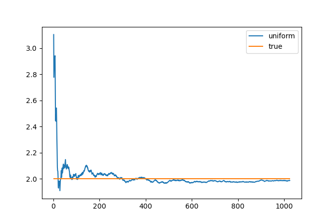
We can see that it indeed converges to the value of \( I = 2 \), but it fluctuates a lot (because it is random).
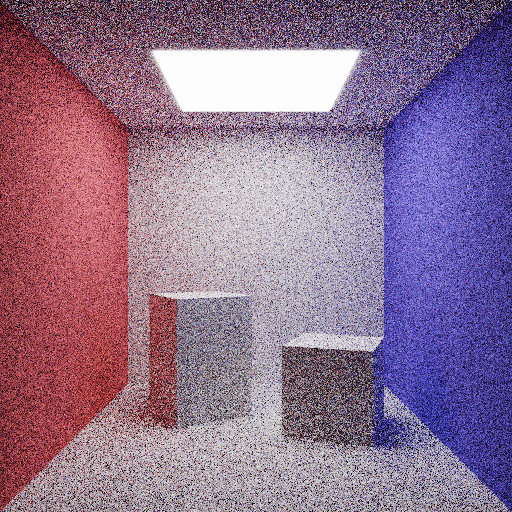
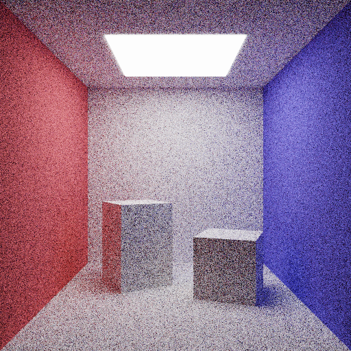
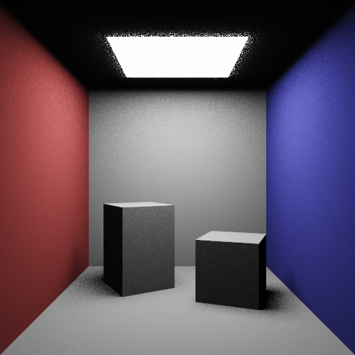
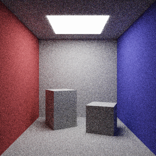
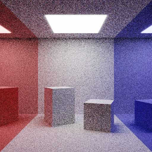
Our next test bed will be a nice diffuse Cornell Box, rendered at 64 samples per pixel (spp) by sampling the incoming light direction \( \omega_{in} \) uniformly on the hemisphere:
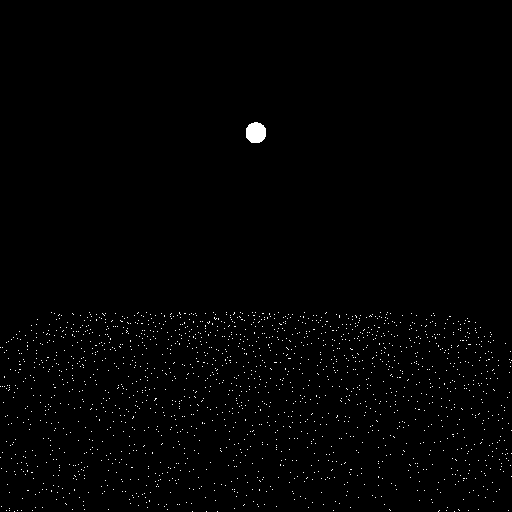
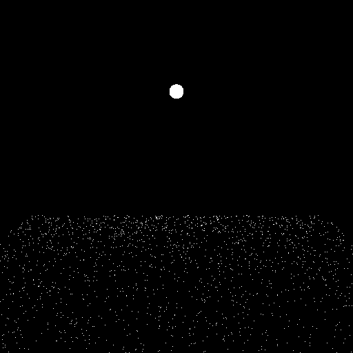
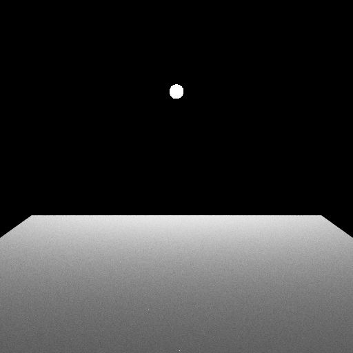
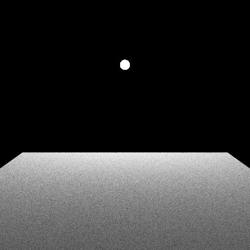
Out final test will actually be a pair of scenes: one (one the left) with a diffuse plane and a small light source, another (on the right) with a metallic plane and a large light source, both rendered with 64 spp and uniform sampling as well:
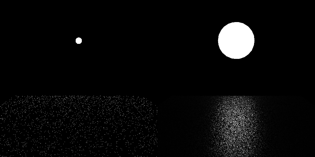
There's so much noise in all these!
Importance sampling
So, we've seen that the result of Monte-Carlo integration is noisy. One obvious way to reduce the noise is to increase the number of samples, but maybe there's a better way?
Remember that we didn't actually need uniform distribution of samples – we can use any distribution, as long as it satisfies some mild assumptions above.
Let's look at the variance again:
\[ \mathbb{Var}[I_{MC}] = \frac{1}{N} \mathbb{Var}\left[ \frac{f(X_1)}{p(X_1)} \right] \]Variance of some value is minimized when this value is constant. In our case, if \( p(x) = C \cdot f(x) \), then \( \frac{f(X)}{p(X} \) would be a constant random variable, having zero variance!
What is the value of C? Well, since \( p(x) \) is a probability distribution, its integral should be equal to 1:
\[ 1 = \int\limits_\Omega p(x) dx = \int\limits_\Omega C\cdot f(x) dx = C \cdot I \]So, if we take \( p(x) = \frac{1}{I}f(x) \), we will get a perfect Monte-Carlo method: it has zero variance, i.e. it immediately gives us the true value of the integral!
But why does this happen? Look at a one-sample Monte-Carlo estimate:
\[ I_{MC} = \frac{f(X_1)}{p(X_1)} = \frac{f(X_1)}{\frac{1}{I}f(X_1)} = I \]In order to actually use this distribution, we need to know the value \( I \) beforehand. But this is the very value we tried to compute! Oops.
So, the perfect probability distribution is actually useless for us, because we cannot compute its PDF \( p(x) \) without knowing the desired integral \( I \) in the first place. However, it gives us an important hint: to reduce variance, we need to make \( p(x) \) look similar to \( f(x) \), so that the fraction \( \frac{f(x)}{p(x)} \) doesn't fluctuate too much and has low variance.
This idea is called importance sampling: trying to sample more important areas more frequently.
Let's apply this idea to our first test case \( \int\limits_0^\pi \sin x dx \). Instead of using uniformly distributed samples on \( [0,\pi] \), let's take a distribution that looks like a parabola centered at \( \frac{pi}{2} \):
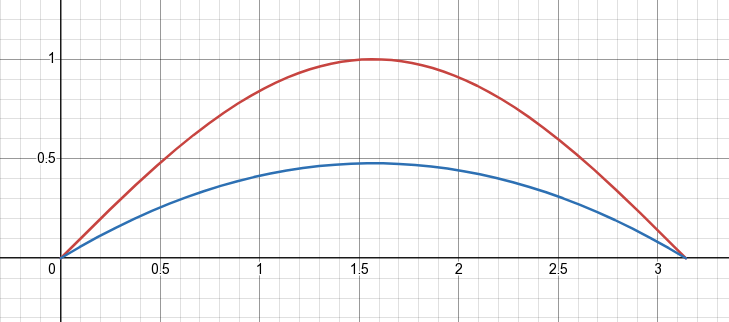
This probability turns out to be equal to
\[ p(x) = \frac{3}{2\pi} \left[ 1 - \left(\frac{2x}{\pi} - 1\right)^2 \right] \]and we can use CDF inversion to sample it. Quite curiously, the CDF turns out to be simply the smoothstep function:
\[ P(X < x) = 3\left(\frac{x}{\pi}\right)^2 - 2\left(\frac{x}{\pi}\right)^3 = \text{smoothstep}\left(\frac{x}{\pi}\right) \]You can find the inverse function on the Inigo Quilez site. Here's what we get using this sampling method, compared to uniform sampling:
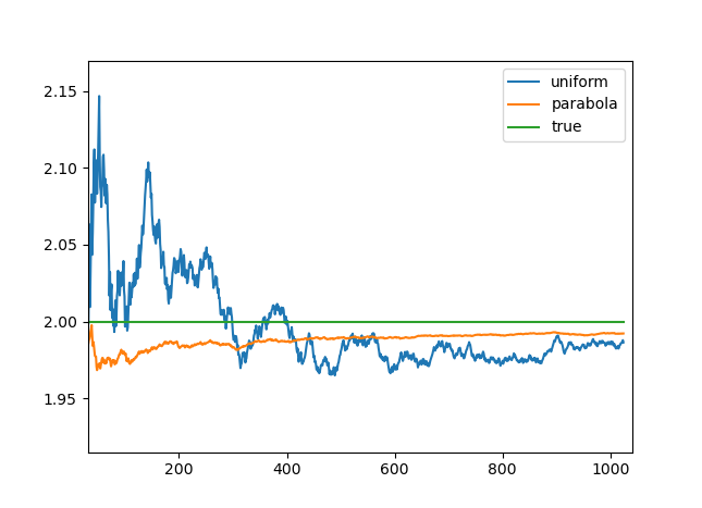
It clearly converges much faster! Let's look at our other examples.
In general, it is pretty hard to figure out a good sampling distribution for use in path tracing, because the integrated function is pretty complicated:
\[ I_{in}(p,\omega_{in})\cdot r(p,\omega_{in},\omega_{out})\cdot (\omega_{in}\cdot n) \]One simple choice that works for diffuse materials (such that \( r=\text{const} \) is to ignore the \( I_{in} \) part and use a distribution proportional to the dot product \( (\omega_{in}\cdot n) \). This distribution is called cosine-weighted hemisphere distribution, because the PDF is proportional to the cosine of the angle between the direction and the surface normal \( n \).
Using this distribution instead of a uniform one, we get a nice (though far from complete) noise reduction:
However, it doesn't help much with our last test scene – neither with the diffuse plane:
nor with the metallic surface:
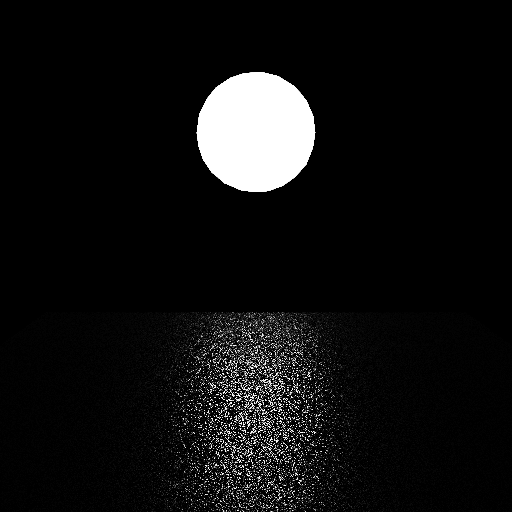
Why so? The answer is quite simple: in these cases, both the uniform distribution and the cosine-weighted one poorly approximate the integrated function:
- For the diffuse surface, they are good approximations of the BRDF term \( r \), but they poorly approximate the incoming light \( I_{in} \) since the light comes only from a handful of directions pointing to the small sphere
- For the metallic surface, they are OK approximations of the incoming light \( I_{in} \) (which now comes from a lot of directions, because the light source is quite big), but they are poor approximations of the BRDF term \( r \), which for nice polished metals wants to reflect light only in a certain direction, and not in a random one
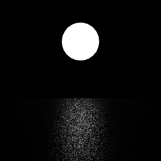
One thing we can do for the metallic plane is to figure out a distribution that sends more rays towards the direction of perfect reflection. This distribution is called VNDF, and here's how it looks compared to the uniform distribution:
We get a very noticeable improvement!
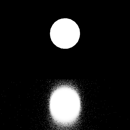
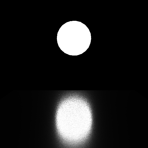
There's something more we can do: send random directions directly to the light source! This is called direct light sampling, or light importance sampling, or just light sampling, something like that. It does wonders for our plane-with-a-sphere scenes:
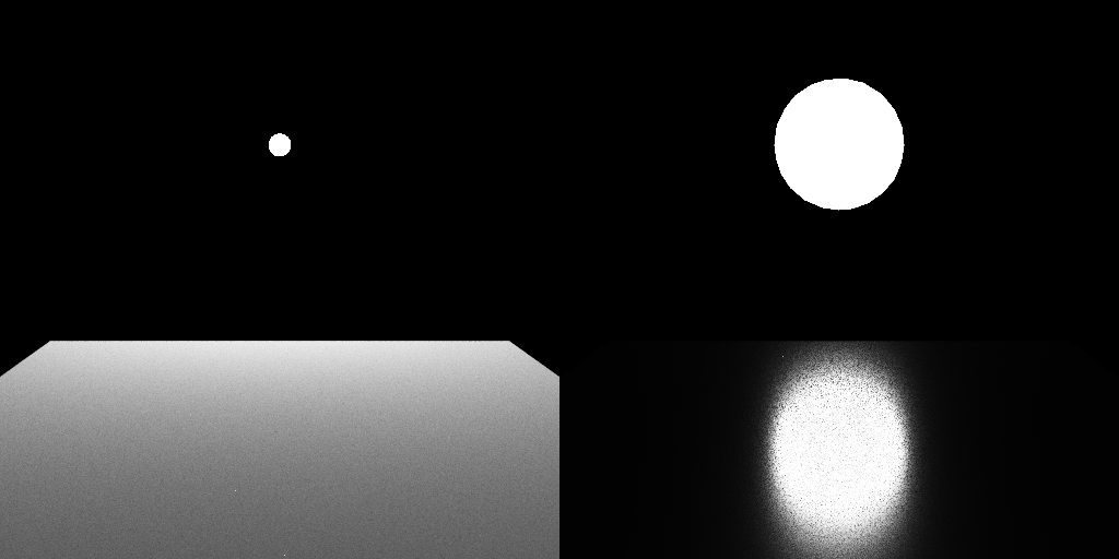
though it is still far from perfect for the metallic surface, since for a large light source there are many directions that are irrelevant for the BRDF (i.e. because the surface wants to reflect in a specific direction, and not in a bunch of directions around it).
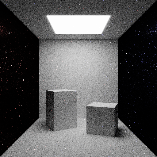
However, it's a bit of a miracle that this approach even works: the only reason for that is that we have an exceptionally simple scene, where \( I_{in} \) is zero in all directions that don't hit a light source directly. In the Cornell box scene, we have a lot of diffuse light spreading around the scene, and using just direction light sampling produces a wrong image:
The reason is that the requirement \( f(x) > 0 \Rightarrow p(x) > 0 \) is not fulfilled for this distribution: there are a lot of directions with non-zero values of our integrated function (namely, the diffuse reflections of light by the objects in the scene), but the distribution only samples a certain subset of directions (those leading directly to a light source).
So, we have a bunch of sampling strategies (i.e. a bunch of distributions), and each of them works in some cases and doesn't work in other cases. It almost sounds like we should combine them somehow!
Multiple importance sampling
We're finally there!
How can we combine several distributions at once? One obvious way would be to, say, each time we generate a sample, select one of the distributions at random and just use it in our calculations.
For example, if we have two distributions \( p_1(x) \) and \( p_2(x) \), we flip a fair coin, and with probability 1/2 our estimator is either
\[ \frac{f(X)}{p_1(X)} \]or
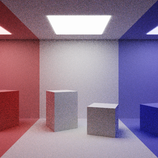
\[ \frac{f(X)}{p_2(X)} \]Using cosine-weighted distribution for \( p_1 \), and direct light sampling for \( p_2 \), we get the following (again, at 64 spp):
It's hard to say if the noise is reduced or not, simply because the image on the right is wrong! It is darker than it should be.
It's easy to see why this happened: in essence, by selecting one of the two distributions at random, our final image is a mix of two images, each produced exclusively by one of distributions. But we know that using only direct light sampling is wrong! So what we got here is a 50-50 mix of a correct and an incorrect image, which is again an incorrect image (even if it is 50% more correct).
We're clearly doing something wrong. Let's return to the basics: for the Monte-Carlo method, if we generate a sample using a distribution \( p(x) \), we need to compute the estimator as
\[ \frac{f(X)}{p(X)} \]What is the probability of generating a sample using the above method? Well, with a 50% change we could generate it using \( p_1 \), and likewise with \( p_2 \), so the real probability of the sample is
\[ p(X) = \frac{1}{2}p_1(X) + \frac{1}{2}p_2(X) \]and this is what we should be dividing by in our Monte-Carlo estimator! So in this case our estimator (for a single sample) is
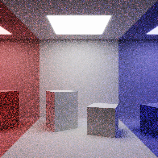
\[ \frac{f(X)}{\frac{1}{2}p_1(X) + \frac{1}{2}p_2(X)} \]This approach is called multiple importance sampling (MIS). If we use this for the Cornell box scene and compare to cosine-weighted distribution only, we get (at 64 spp):
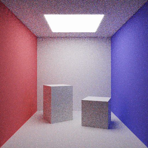
We can see that the noise is severely reduced! It is still quite noisy, but hey, that's just 64 samples :)
We can apply this to our plane-with-a-light scenes. This time, we'll use 3 different distributions with equal probabilities:
- Cosine-weighted distribution, which is good for the diffuse part
- VNDF distribution, which is good for the specular part
- Direct light sampling, which is always good, but wrong if used without anything else
What we get (on the right) is slightly worse than using direct light sampling in these scenes:
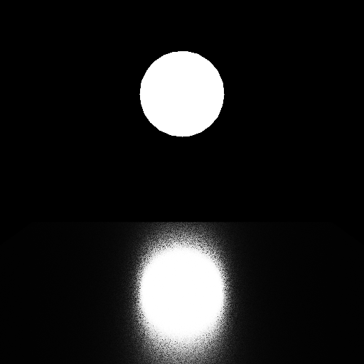
again, because these scenes are intenionally very simple and lack any diffuse light. However, if we take a more complicated scene with both diffuse and metallic surfaces, MIS (on the right) is noticeably better than using, say, just VNDF (on the left), this time with 256 samples:
or compared to just a cosine-weighted distribution, which is completely useless for reflective surfaces:
We can also take a smarter approach and choose different probabilities for each strategy based on material properties. For example, for rough materials we probably need cosine-weighted distribution \( p_{cosine} \) and direct light sampling \( p_{light} \), while for smooth materials we're better use the VNDF \( p_{vndf} \) for sampling directly the reflected direction. So, given roughness \( \sigma \), we can take the distribution
\[ \sigma \left(\frac{1}{2} p_{cosine} + \frac{1}{2} p_{light}\right) + (1 - \sigma) p_{vndf} \]and it gives even more improvement compared to MIS with equal weights:
In general, if you have a bunch of sampling strategies \( \{p_1\dots p_M\} \), and for each sample you use on of them with some probability \( w_i \) (of course, \( \sum w_i = 1 \)), your final probability of choosing a sample is
\[ p(X) = \sum w_i p_i(X) \]and your (one-sample) Monte-Carlo estimator is
\[ \frac{f(X)}{\sum w_i p_i(X)} \]Notice how, even though we generated a sample using just one distribution, we still need to compute the probability of generating this sample by all distributions, in order for this method to work correctly.
The only requirement for MIS to work is that, as always in Monte-Carlo integration, we need \( f(x) > 0 \Rightarrow p(x) > 0 \). Our \( p(x) \) is a mix of \( p_i(x) \), and it is greater than zero as long as at least one of our distributions has nonzero pdf at every point:
\[ f(x) > 0 \,\Rightarrow \,\exists i : p_i(x) > 0 \]This is why a mix of direct light sampling and, say, cosine-weighted sampling works: even though one of the distributions fails to produce some important samples, we're good as long as at least one distribution can produce this sample.
Light sampling with MIS
There's a catch when using direct light sampling inside multiple importance sampling. Typically, when you have many lights (e.g. light-emitting triangles), you might select one of them at random, pick a random point on its surface, and set your direction sample to point in the direction of this point. However, for MIS to work, we need to compute the probability of generating a direction sample using all our distributions. This means that we need to compute the probability of generating this sample by every light source!
This ultimately boils down to sending a ray in this direction and finding all light sources that intersect this ray. Not just the closest hit, but all of them. If you're doing some raytracing, you probably want a BVH for that, or even a separate BVH just for the light sources (this is what students do in my course).
This can be seen as an instance of MIS inside MIS. Our top-level MIS is composed of, say, two distributions: one for the material (BRDF) of the surface, and one for the light sources. The latter is itself a MIS combining individual distributions pointing towards individual light sources.
Stratified sampling
Stratified sampling is a technique which subdivides the original integration domain into some disjoint sections
\[ \Omega = \coprod \Omega_i \](Here, \( \coprod \) is the disjoint union.)
Then we generate a sample in each of this sections \( X_i \in \Omega_i \) using some distribution \( p_i \) supported on this section, meaning it has zero probability outside of it.
Then the Monte-Carlo estimate is given by
\[ I_{MC} = \sum \frac{f(X_i)}{p_i(X_i)} \]But wait, we know that this is a wrong formula! We should sum the probabilities, instead of just using one of them! And where's the \( \frac{1}{N} \) factor?
Well, actually we're secretely summing the probabilities already. Each \( p_i \) is nonzero on its own section \( \Omega_i \) of the whole domain \( \Omega \), so for each point \( X \in \Omega \) only one of the \( p_i \) can be nonzero. Since we generated \( X_i \) using \( p_i \), we know that \( p_i \) is the one distribution having nonzero probability at \( X_i \), and all the others are zero.
However, since we're still using \( N \) different sampling strategies (one for each section \( \Omega_i \)), we can pretend that we're selecting them at random, each with probability \( \frac{1}{N} \), this the final probability of the sample \( X_i \) is
\[ p(X_i) = \frac{1}{N}p_i(X_i) \]and the N-sample Monte-Carlo estimator is
\[ I_{MC} = \frac{1}{N}\sum\frac{f(X_i)}{p(X_i)} = \frac{1}{N}\sum\frac{f(X_i)}{\frac{1}{N}p_i(X_i)} = \frac{1}{N}\cdot N\cdot\sum\frac{f(X_i)}{p_i(X_i)} = \sum\frac{f(X_i)}{p_i(X_i)} \]So, stratified sampling can be seen as kind of a special case of multiple importance sampling. Kind of, because pretending that something non-random (using one sample from each \( \Omega_i \)) is actually random (selecting a random \( \Omega_i \) and its \( p_i \)) is sketchy. The proper derivation of stratified sampling simply partitions the integration domain and represents the integral as a sum
\[ I = \sum I_i = \sum\limits_i \int\limits_{\Omega_i}f(x)dx \]and uses a single-sample Monte-Carlo estimator in each of the sections. Still, I think this is a fun and curious connection :)
Veach'97 thesis
Now, what's with the Veach's thesis that introduced this technique? If we go to part II, section 9.2 of the thesis, which is literally titled "Multiple importance sampling", we see something weird, involving generating several samples \( X_{ij} \) using each of the sampling strategies \( p_i \), and mixing them with some weights \( w_i \). The final formula for the estimator
\[ \sum\limits_i^N \frac{1}{N_i} \sum\limits_j^{N_i} w_i(X_{ij})\frac{f(X_{ij})}{p_i(X_{ij})} \]doesn't even look like a Monte-Carlo estimator – it has some extra terms in it!
The explanation is rather simple: Veach consideres a more general scenario, where you decide on the number of samples for each stratagy beforehand, and then use this formula for the integral.
If we take the weights \( w_i \) acording to the balance heuristic described in the same section of the thesis, and use the one-sample estimator described in section 9.2.4 "One-sample model", we arrive at the very sample formula for multiple importance sampling that we derived earlier in this article.
End section
So, this was a lot of text and images and formulas, but I hope you've learnt the most important thing in this article:
To properly apply multiple importance sampling, we need to add up the probabilities of generating a sample by all of our sampling strategies, and use it in the denominator of the Monte-Carlo estimator.
I could just tweet this sentence, but where's the fun in that, huh? :)
Here's an article in Ray Tracing Gems II about multiple importance sampling, if you want to read more about it.
And, as always, thanks for reading.