I was reading something about quiver representations and some proof started with take any vector not orthogonal to any of these N vectors
. This seems trivial, but...cut can you actually always do that?
Contents
Intuition
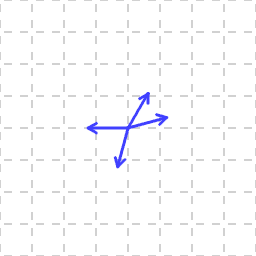
I mean, obviosly you can! Say, you have a bunch of (non-zero) vectors:
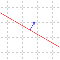
In 2D, the vectors orthogonal to a single vector form a line through the origin:
If we do this for all our vectors, we get a union of lines:
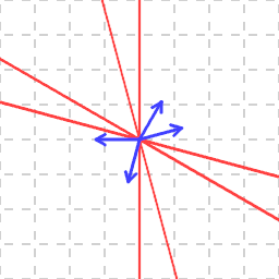
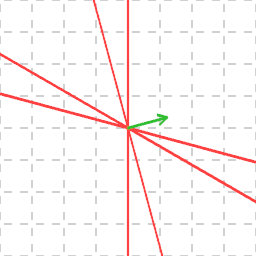
And the question now is: can we find a vector not on any of the red lines (i.e. in the white area)? It's visually obvious that yes indeed we can — pretty much a random vector will do:
The same works for any dimension \(\geq 2\). E.g. in 3D you'd get a union of a finite set of planes through the origin, and you just need to find a vector not in any of these planes.
In 1D things are a bit stupid: any two non-zero vectors are collinear and cannot be orthogonal, so you can just pick any non-zero vector — it won't be orthogonal to any of your input vectors.
However, it is often the case in math that a visually obvious fact can be notoriously hard to prove, or even turn out to be false in higher dimensions.
So how can we prove this?
Measure-theoretic proof
Let's try to formalize the intuition. The idea is that lines occupy a small portion of the space, and there's still a ton of space left if we exclude a finite set of lines. Let's take the (K-dimensional!) volume of the space and subtract the volume of the subspaces orthogonal to each of the input vector. The problem is that, last time I checked, the whole space was infinite, and subtracting something from infinity is usually a shady idea at best (you can get to things like \(\infty - \infty = \infty\)).
So, instead let's bound our space. Let's say we're only interested in the resulting vectors with length no larger than \(1\). In other words, we're interested in what happens inside a ball with radius \(1\). The exact measure (aka K-dimensional volume) of this ball isn't relevant to us, it's OK to just know that it's non-zero.
A subspace (line/plane/etc) orthogonal to some input vector cuts away a certain smaller-dimensional ball, — e.g. in 3D we'd have a 2D plane cutting through a 3D ball and resulting in a 2D circle (with interior) of forbidden
vectors. What we want is some vector inside the big ball but not inside one of those balls of smaller dimension.
But those smaller balls have measure (volume) zero! A simple way to prove this is to wrap them into a (K-dimensional) box with one axis parallel to an input vector and all other axes orthogonal to it (and thus parallel to the forbidden
ball). E.g. in 3D we can take a circle of forbidden vectors corresponding to one input vector and take a bounding square. However, we have 3 dimensions, so we extend this square a bit along the normal to the circle, which is parallel to the input vector (which in turn is orthogonal to the circle, rememeber?), and we can extend it by any non-zero amount to get a proper 3D box. In particular, we can extend it by smaller and smaller amounts, — leading to smaller and smaller volumes of this box, — while still containing the forbidden
circle.
Now, if a set (the forbidden
circle) is contained in each of a sequence sets (the boxes) with volume converging to zero (because their height converges to zero), it itself has volume zero (this follows from the basic properties of a measure). This is all to say that those smaller-dimensional balls have measure (aka volume) zero, simply because they live in a subspace of smaller dimension.
A union of (a finite collection of) sets of measure zero again has measure zero, and the measure of the set of allowed
vectors — that is, the unit ball excluding the forbidden
vectors — is thus some positive number (volume of the K-dimensional ball) minus zero, which is still that positive number. A set with positive measure cannot be empty, thus there exists a vector not in one of the forbidden sets. Hurray!
The proof is a bit involved if you've never worked with measure theory; on the other hand, it probably sounds trivial if you've taken a proper analysis class. In any case, it captures the essence of our intuition: there does exist a vector not orthogonal to a set of input vectors simply because those vectors orthogonal to any of the input vector form a tiny (lower-dimensional) subset of the whole space.
However, I'm not really satisfied with this proof. Firstly, it feels like a huge overkill to use measure theory to something that talks about simple geometry. Secondly, it doesn't work for other number fields! E.g. it doesn't work if I'm only interested in vectors with rational coefficients, or even coefficients from a finite field!
And if you thing that vectors with coefficients in a finite field is some useless toy for algebraists to play with, I regret to inform you that modern cryptography is literally based on finite-field geometry.
Probabilistic proof
That's not really a separate proof, just a reinterpretation of the measure-theoretic one. Take a random vector inside the unit ball (or on the unit sphere, whichever you prefer). By the previous section, the probability that it will be orthogonal to one of the input vectors is zero (volume of the union of circles cut by hyperplanes — which is zero — divided by the volume of the ball). So, a random vector already satisfies our requirement.
Algebraic proof
Let's think in formulas. If I have a 2D vector \(v = (v_x, v_y)\), the set of vectors \(r = (x, y)\) orthogonal to it satisfy the equation \(\langle v, r \rangle = 0\), or in coordinates
\[ x\cdot v_x + y\cdot v_y = 0 \](I use the angle brackets \(\langle\cdot,\cdot\rangle\) to denote the dot product.)
In 3D, it would be
\[ x\cdot v_x + y\cdot v_y + z\cdot v_z = 0 \]and so on. Because we have a bunch of input vectors \(v_i\), each one will get its own equation \(\langle v_i, r\rangle=0\), or in coordinates
\[ x\cdot v_{i,x} + y\cdot v_{i,y} + z\cdot v_{i,z} = 0 \]Now, if we have a set of equations like \(f_i(r)=0\), we can multiply them all:
\[ F(r) = f_1(r)\cdot f_2(r)\cdot\dots\cdot f_N(r) = 0 \]and the solutions to this multiplied equation will be exactly the solutions to one of the original equations \(f_i(r)=0\) (because a product is zero precisely when one of the multiples is zero).
So, what we're asking is if there exists a vector \(r\) such that \(F(r)\neq 0\). This is equivalent to asking whether \(F(r)\) is just the zero function, i.e. the zero polynomial. But of course it isn't the zero polynomial: we've multiplied together a bunch of non-zero polynomials (like \( x\cdot v_x + y\cdot v_y + z\cdot v_z \)), so the result is a non-zero polynomial, so it cannot be zero everywhere!
Now, I bet you've never really thought about it unless you've studied abstract algebra, but
- Why multiplying non-zero polynomials gives you a non-zero polynomial (maybe something can cancel out?), and
- Why a non-zero polynomial cannot evaluate to zero everywhere?
Concerning 1, it's true that some coefficients might cancel out, e.g. in \((x+y)(x-y)=x^2-y^2\) the coefficient of \(xy\) cancels out, but it never happens that everything cancels out, it must be that some of the factors was a zero polynomial itself! For example, take
\[ (ax+by)(cx+dy) = ac\cdot x^2 + (ad+bc)\cdot xy + bd\cdot y^2 \]The coefficient at \(x^2\) can be zero only if \(a\) or \(c\) is zero. If \(a\) is zero, then \(b\) is non-zero (otherwise the left factor \(ax+by\) is a zero polynomial). Then, if the coefficient at \(y^2\) is zero, then either \(b\) or \(d\) is zero. \(b\) cannot be zero together with \(a\), so \(d\) must be zero, and thus \(c\) non-zero and thus the coefficient at \(xy\) is just \(bc\), both of which are non-zero, so the product is a non-zero polynomial (i.e. at least one coefficient not zero). If otherwise \(a\) is not zero, but \(c\) is zero, then \(d\) is non-zero, etc etc.
You can do the same reasoning for any number of variables and any degree of the polynomials being multiplied, but it gets messy really quickly. The usual proof does something clever instead: recognize that a polynomial in \(N\) variables is the same as a polynomial in \(1\) variable, with coefficients themselves being polynomials of the other \(N-1\) variables! Then if the product of non-zeros is non-zero
is true for the coefficients (which are polynomials in \(N-1\) variables now), then it is true for polynomials in \(N\) variables: in a product
simply look at the coefficient at the highest term \(x^{n+m}\), which is \(a_n(y,z)\cdot b_m(y,z)\) — it is non-zero provided that the individual coefficients \(a_n\) and \(b_m\) are non-zero.
The algebraic structures where the product of non-zeros is non-zero are so special that they have their own name: integral domains. What we've just proved, — or, rather, sketched the proof of, — is the fact that polynomials with coefficients in an integral domain themselves form an integral domain.
Ok, so point 1 is just some basic but clever abstract algebra. What about point 2?
Polynomials vs polynomial functions
This distinction is rarely mentioned in maths classes, unless one is learning some abstract algebra. The reason is that, when you're working with infinite fields of numbers (e.g. rational/real/complex numbers), there is no distinction: polynomials (as abstract formulas defined by their lists of coefficients) and polynomial functions (functions that are defined by a polynomial formula) are in 1-to-1 correspondence. The real-valued function defined by \(f(x,y) = x^2-y^2\) cannot be defined by a polynomial with a different set of coefficients.
The usual proof uses the fact that a polynomial can only have a finite number of roots, together with induction on the number of variables. Since an infinite field has an infinite number of elements, a non-zero polynomial cannot be zero everywhere. But this arguments doesn't work for finite fields!
Consider \(\mathbb F_2\), the field with just two elements \(\{0,1\}\) and the (only possible) addition rule \(1+1=0\). This is also known as arithmetic\(\mod 2\). Consider the polynomial \(f(x)=x+x^2\). Compute it for all possible numbers
, i.e. elements of the field:
So, as a function, this polynomial is identically zero! However, the polynomial itself — as a formula defined using only additions and multiplications — is non-zero: two of it's coefficients (namely, those at \(x\) and \(x^2\)) are non-zero. Oops!
There's another way to see this. We know that, if I want a polynomial with roots \(x_1, \dots, x_n\), I can just multiply out monomials of the form \((x-x_1)\), \((x-x_2)\), \(\dots\), \((x-x_n)\), and I'll get a polynomial \(f(x) = (x-x_1)\cdot\dots\cdot(x-x_n)\) which will have all these numbers as roots. Now, in a finite field, I can list all the elements of the field \(\{x_i\}\), and just make a polynomial \(\varphi(x)\) with all the elements as roots. Of course, it will evaluate to zero everywhere, by construction. In fact, any polynomial which turns out to be a zero function must be a multiple of \(\varphi(x)\). In particular, it must have degree at least as large as the size of the underlying field of numbers that we're working with.
What does it tell us about the algebraic proof above? Because the polynomial \(F(r)\) we've constructed has degree \(N\) (the number of input vectors), the proof still works as long as the field of scalars we're working with has more than \(N\) elements in it. For example, the proof still works if I'm interested in \(N=4\) vectors, provided that the coefficients are from \(\mathbb F_5\) (arithmetic\(\mod 5\)). For infinite fields, the proof always works.
Explicit algorithm
That's too much math, I just want an explicit algorithm to find such a vector, and I'm not happy with a probabilistic algorithm — after all, when working with floating-point numbers, zero probabilities turn into very small but non-zero probabilities.
Fine, here you go! Let's build a vector that is not orthogonal to all input vectors \(\{v_i\}\) step by step. At each step, let \(\{r_k\}\) denote the vector we've already computed, which is not orthogonal to all input vectors with indices \(\leq k\).
Step \(1\): take \(r_1 = v_1\). As the input vectors are non-zero, the dot product \(\langle r_1, v_1\rangle = |v_1|^2\) is just the squared length, thus non-zero, thus the vectors are not orthogonal (in other words, a vector is not orthogonal to itself).
Step \(k\): take \(r_k = r_{k-1} + \lambda v_k\). How do we find \(\lambda\)? Well, for each input vector with index \(i\leq k\), we want the dot product \(\langle r_k, v_i\rangle\) to be non-zero:
\[ \langle r_k, v_i\rangle = \langle r_{k-1} + \lambda v_k, v_i\rangle = \langle r_{k-1}, v_i\rangle + \lambda \langle v_k, v_i\rangle \neq 0 \] \[ \Longrightarrow \lambda \langle v_k, v_i\rangle \neq -\langle r_{k-1}, v_i\rangle \]For \(i< k\), the right-hand size \(-\langle r_{k-1}, v_i\rangle\) is always non-zero by induction. If for some \(i\) we have \(\langle v_k, v_i\rangle=0\), then the inequality is already satisfied (zero is not equal to something non-zero). Otherwise, we have a forbidden value of \(\lambda\):
\[ \Longrightarrow \lambda \neq -\frac{\langle r_{k-1}, v_i\rangle}{\langle v_k, v_i\rangle} \]Similarly, at step \(i=k\), we know that \(\langle v_k, v_k\rangle\) is non-zero (because the input vectors are non-zero), so we get another forbidden value of \(\lambda\):
\[ \Longrightarrow \lambda \neq -\frac{\langle r_{k-1}, v_k\rangle}{\langle v_k, v_k\rangle} \]Thus, at step \(k\), we'll have at most \(k\) such forbidden values, and we can simply pick any number not equal to any of the forbidden values at this step. For example, when working with rational/real numbers, you can track the largest forbidden value, and then take this value \(+1\) as your value for \(\lambda\).
After \(N\) steps, you'll have a vector not orthogonal to any of the input vectors, guaranteed. Hurray!
Notice that if your number field has \(k\) elements, then you might fail at step \(k\), as you'll not be able to find a number not equal to any of the forbidden values, in line with what we've talked about in the previous section. I said might fail, because some of the forbidden values might turn out to be equal to each other! I still don't know if this is a strict bound, though :)
This algorithm has quadratic time complexity, so I'd still recommend generating a random vector and testing if it's orthogonal to any of the input vectors — it probably isn't :)