In my raytracing course at SPbU there's a lecture dedicated to importance sampling (because without it any raytraced scene is either too noisy or complete garbage, depending on the materials used). It is well-known that importance sampling can reduce the variance (aka noise) of the result, but I've never seen any specific estimates or guarantees on how the variance will be reduced. So, naturally, I ended up deriving my own :)
Contents
Monte-Carlo TL;DR
Monte-Carlo integration is a probabilistic method for computing integrals that works best when the integrated function is particularly nasty, or when the integration domain is high-dimensional (like in raytracing), where most other methods fail miserably. See also my other article with a more in-depth discussion of Monte-Carlo method in raytracing specifically.
It works like this. Say, we want to compute the integral of a function \(f(x)\) over some domain \(\Omega\). The domain \(\Omega\) is largely irrelevant here; it can be a 1D inteval, a 2D shape, a hemisphere, etc. To compute the integral, we draw \(N\) random samples \(X_i\) from some probability distribution \(p(x)\) over \(\Omega\) and estimate the value of the integral as
\[ I = \int\limits_\Omega f(x)dx \approx \frac{1}{N}\sum \frac{f(X_i)}{p(X_i)} \]Intuitively, we compute function values at random points, but if the point is rare (low probability), we take its value with higher weight (divide by probability) to compensate for rarity. Then we average over many such samples to get a better estimate.
With this method, we get the desired value \(I\) on average. To prove that, compute the expected value of the estimator, using the fact that all \(X_i\) are independent and identically distributed (iid), and so are \(\frac{f(X_i)}{p(X_i)}\):
\[ \mathbb E \left[\frac{1}{N}\sum \frac{f(X_i)}{p(X_i)}\right] = \frac{1}{N}\sum \mathbb E \left[\frac{f(X_i)}{p(X_i)}\right] = \\ = \frac{1}{N}\cdot N\cdot \mathbb E \left[\frac{f(X_1)}{p(X_1)}\right] = \int\limits_\Omega \frac{f(x)}{p(x)} p(x)dx = \int\limits_\Omega f(x)dx = I \]In essence, all terms in the sum have the same distribution, so the expected value of their average is the same as the expected value of each single sample. Then, we compute the expected value by definition; it involves multiplying by probability \(p(x)\), which conveniently cancels out with the \(\frac{1}{p(x)}\) in our estimator, and we're left with just the desired integral.
The result is correct on average, meaning that we always get something noisy. To estimate the amount of noise, compute the variance of the estimator, again using that all samples are iid:
\[ \mathrm{Var}\left[\frac{1}{N}\sum \frac{f(X_i)}{p(X_i)}\right] = \frac{1}{N^2}\sum \mathrm{Var}\left[\frac{f(X_i)}{p(X_i)}\right] = \\ = \frac{1}{N^2}\cdot N \cdot \mathrm{Var}\left[\frac{f(X_1)}{p(X_1)}\right] = \frac{1}{N}\cdot \mathrm{Var}\left[\frac{f(X_1)}{p(X_1)}\right] \]Now, the value \(\mathrm{Var}\left[\frac{f(X_1)}{p(X_1)}\right]\) depends only on the function \(f(x)\) and our chosen probability distribution \(p(x)\), but it doesn't depend on \(N\), so it's just some problem-specific constant. The \(\frac{1}{N}\) factor is important, though. Let's compute the standard deviation of the estimator as the square root of variance:
\[ \sigma = \frac{1}{\sqrt N}\cdot \sqrt{\mathrm{Var}\left[\frac{f(X_1)}{p(X_1)}\right]} \]Whatever this large square root on the right is equal to, it doesn't matter, since it's just a constant. The important thing is \(\frac{1}{\sqrt N}\) — it tells us what the error of the method is.
Since \(\frac{1}{\sqrt N}\) tends to zero as \(N\) tends to infinity, it means that the method indeed converges to the true result as we get more samples (i.e. the noise goes to zero). However, the convergence is rather slow because of that square root: to have a 2x better image (i.e. to reduce noise by 2x), we need to get 4x more samples! This is sad.
Importance sampling TL;DR
Taking more samples is one way of reducing the noise (i.e. reducing variance). The other method is to reduce the variance of a single sample, i.e. the quantity
\[ \mathrm{Var}\left[\frac{f(X)}{p(X)}\right] \]by choosing the probability distribution \(p(x)\) of our samples in a clever way. Let's explicitly compute this variance, using the formula \(\mathrm{Var}(X) = \mathbb E [X^2] - \mathbb E [X]^2\):
\[ \mathrm{Var}\left[\frac{f(X)}{p(X)}\right] = \mathbb E \left[\frac{f^2(X)}{p^2(X)}\right] - \mathbb E\left[\frac{f(X)}{p(X)}\right]^2 = \\ = \int\limits_\Omega \frac{f(x)^2}{p(x)^2}p(x)dx - I^2 = \int\limits_\Omega \frac{f(x)^2}{p(x)}dx - I^2 \]Here I'll use one stupid trick: rewrite \(I^2\) as \(I\cdot I\) and replace only one of the \(I\)'s with its definition as the integral of \(f(x)\):
\[ \mathrm{Var}\left[\frac{f(X)}{p(X)}\right] = \int\limits_\Omega \frac{f(x)^2}{p(x)}dx - I^2 = \int\limits_\Omega \frac{f(x)^2}{p(x)}dx - I\cdot\int\limits_\Omega f(x)dx = \\ = \int\limits_\Omega \left( \frac{f(x)^2}{p(x)} - I\cdot f(x)\right)dx = \int\limits_\Omega I\cdot f(x) \cdot \left( \frac{f(x)}{I\cdot p(x)} - 1\right)dx \]We can see that if we could guarantee that \(\frac{f(x)}{I\cdot p(x)} = 1\), the expression in parentheses becomes zero, and the variance becomes zero! From this equation, we can explicitly find \(p(x)\):
\[ \frac{f(x)}{I\cdot p(x)} = 1 \Longrightarrow p(x) = \frac{f(x)}{I} \]I will call this the ideal probability distribution \(p^*(x)\), and I'll denote the samples from this distribution as \(X^*\). With this distribution, the variance of a single sample is zero! Meaning that we get the correct answer with just one sample. Sounds suspicious, doesn't it?
Look closer: to use this in Monte-Carlo integration, we need to compute the probability \(p^*(X^*)\) of a sample, which equals \(\frac{f(X^*)}{I}\). Given that we assumed that we know how to compute \(f(X^*)\), it means that we also need to know the value of \(I\) to compute this probability. But the value of \(I\) is exactly what we are trying to compute in the first place!
So, the ideal distribution is kinda useless, since it requires knowing the desired integral in the first place. However, it's not completely useless! It still hints us that if our distribution \(p(x)\) is at least somewhat close to \(p^*(x)\), the value of \(\frac{f(x)}{I\cdot p(x)} - 1\) should still be close to zero, and we still should get some variance reduction.
Some variance reduction sounds promising, but how much exactly is some?
Computing variance reduction (approximately)
We'll compute the variance reduction as a function of the relative difference \(\varepsilon(x)\) between our chosen distribution \(p(x)\) and the ideal one \(p^*(x)\):
\[ p(x) = p^*(x) \cdot (1 + \varepsilon(x)) \]In other words
\[ \varepsilon(x) = \frac{p(x)-p^*(x)}{p^*(x)} \]We could define the difference in a ton of other ways (e.g. take absolute instead of relative difference, multiply by \(I\) or \(f(x)\) somewhere, etc); however, I've found that this particular form leads to nicer formulas and easier interpretation. It also makes \(\varepsilon(x)\) a unitless quantity, making it easier to reason about.
Note that, since both \(p(x)\) and \(p^*(x)\) are probability distributions, their integral over the whole domain \(\Omega\) is equal to 1, and thus
\[ 1 = \int\limits_\Omega p(x)dx = \int\limits_\Omega \left[p^*(x) + p^*(x)\varepsilon(x)\right] dx = \\ = \int\limits_\Omega p^*(x)dx + \int\limits_\Omega p^*(x)\varepsilon(x)dx = 1 + \int\limits_\Omega p^*(x)\varepsilon(x)dx \]meaning that
\[ \int\limits_\Omega p^*(x)\varepsilon(x)dx = 0 \]Recall that \(p^*(x) = \frac{f(x)}{I}\), and let's compute the single-sample variance:
\[ \mathrm{Var}\left[\frac{f(X)}{p(X)}\right] = \int\limits_\Omega I\cdot f(x) \cdot \left( \frac{f(x)}{I\cdot p(x)} - 1\right)dx = \int\limits_\Omega I^2\cdot \frac{f(x)}{I} \cdot \left( \frac{f(x)}{I\cdot p^*(x)(1+\varepsilon(x))} - 1\right)dx =\\ = I^2 \int\limits_\Omega p^*(x) \cdot \left( \frac{1}{1+\varepsilon(x)} - 1\right)dx \]From here, let's assume that \(\varepsilon(x)\) is small enough, so that we can use the power series \(\frac{1}{1+a} = 1-a+a^2-a^3+\dots\), and also ignore all terms after the quadratic one:
\[ \frac{1}{1+\varepsilon(x)} - 1 = (1 - \varepsilon(x)+\varepsilon(x)^2-\dots) - 1 \approx - \varepsilon(x) + \varepsilon(x)^2 \]Substitute into the integral above to get:
\[ I^2 \int\limits_\Omega p^*(x) \cdot \left( \frac{1}{1+\varepsilon(x)} - 1\right)dx \approx I^2 \int\limits_\Omega p^*(x) \cdot (- \varepsilon(x) + \varepsilon(x)^2)dx = \\ = - I^2 \int\limits_\Omega p^*(x) \varepsilon(x) dx + I^2 \int\limits_\Omega p^*(x) \varepsilon(x)^2dx \]We know that the first integral is zero, so the only thing that's left is
\[ \mathrm{Var}\left[\frac{f(X)}{p(X)}\right] \approx I^2 \int\limits_\Omega p^*(x) \varepsilon(x)^2dx \]which can be interpreted as the expected value of \(\varepsilon(x)^2\) with respect to probability distribution \(p^*(x)\), which I'll denote as \(\mathbb E\left[\varepsilon(X^*)^2\right]\). The value
\[ \int\limits_\Omega p^*(x) \varepsilon(x) dx = 0 \]can be interpreted in the same vein as the expected value \(\mathbb E\left[\varepsilon(X^*)\right]\) of \(\varepsilon(x)\) wrt the probability \(p^*(x)\). Because it is zero, we can derive
\[ \mathrm{Var}\left[\frac{f(X)}{p(X)}\right] \approx I^2 \cdot \mathbb E\left[\varepsilon(X^*)^2\right] = I^2 \cdot \mathrm{Var}\left[\varepsilon(X^*)\right] \]Thus, the variance of our Monte-Carlo estimator is approximately equal to \(I^2\) times the variance of the relative difference between our chosen probability distribution and the ideal one. That is, the more our samples differ from the ideal distribution, the more noise we get! This is something known in raytracing literature, but here we've derived an actual formula.
By the way, the \(I^2\) factor is expected: if you multiply the value of the integral by 10, it is reasonable to expect that the amplitude of noise would also get 10x larger in absolute value.
Computing variance reduction (exactly)
Ok, this previous formula was derived under the assumption that \(\varepsilon(x)\) is sufficiently small. What if we don't want to make any assumptions?
We can still try to rewrite \(\frac{1}{1+\varepsilon}-1\) using the power series, drop the \(-\varepsilon\) term (because the integral of \(p^*(x)\varepsilon(x)\) is zero) which I'll denote with an arrow \(\rightarrow\), and then recognize the same power series once again:
\[ \frac{1}{1+\varepsilon(x)}-1 = (1-\varepsilon(x)+\varepsilon(x)^2-\varepsilon(x)^3+\varepsilon(x)^4-\dots) - 1 \quad\rightarrow \\ \rightarrow\quad \varepsilon(x)^2-\varepsilon(x)^3+\varepsilon(x)^4-\dots = \varepsilon(x)^2\cdot(1-\varepsilon(x)+\varepsilon(x)^2-\dots) = \\ = \frac{\varepsilon(x)^2}{1+\varepsilon(x)} \]However, the power series only works when \(|\varepsilon(x)|<1\). It turns out that we don't need the power series expansion to derive this formula: just add \(\varepsilon(x)\) to the original and combine the fractions:
\[ \frac{1}{1+\varepsilon(x)}-1 \quad\rightarrow\quad \frac{1}{1+\varepsilon(x)} - 1 + \varepsilon(x) = \frac{1}{1+\varepsilon(x)} - \frac{(1-\varepsilon(x))(1+\varepsilon(x))}{1+\varepsilon(x)} = \\ = \frac{1-(1-\varepsilon(x)^2)}{1+\varepsilon(x)} = \frac{\varepsilon(x)^2}{1+\varepsilon(x)} \]So, here's a better, non-approximate formula: the variance of the Monte-Carlo estimator depends on the relative difference \(\varepsilon(x)\) between the chosen and the ideal sample distributions as
\[ \mathrm{Var}\left[\frac{f(X)}{p(X)}\right] = I^2 \cdot \mathbb E\left[\frac{\varepsilon(X^*)^2}{1+\varepsilon(X^*)}\right] = I^2\int\limits_\Omega p^*(x)\frac{\varepsilon(x)^2}{1+\varepsilon(x)}dx \]Numerical experiments
Let's try these estimates with an actual, albeit artificial, example. I'll compute the integral \(\int\limits_0^\pi \sin x\,dx\) with the Monte-Carlo method using two distributions: the uniform distribution \(U(0,\pi)\), and a distribution that looks like a quadratic function symmetric around \(x=\frac{\pi}{2}\) and going to zero at the endpoints \(x=0,x=\pi\). See my other article for exact PDF and CDF formulas for that second distribution.
Here's how their probability densities look like, compared to the ideal distribution:
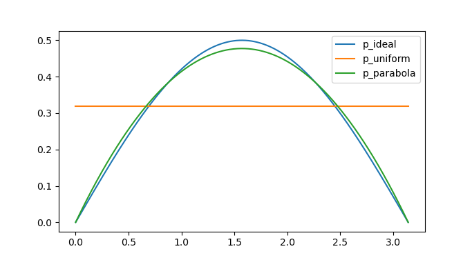
And here's the congervence plot, i.e. the value of the Monte-Carlo estimate after N samples:
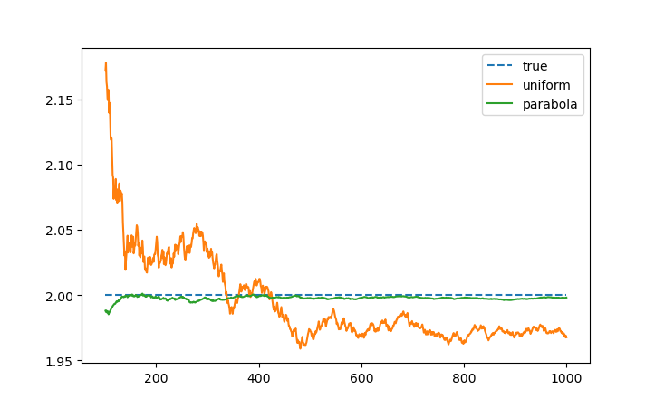
Both seem to converge to the true value, with the quadratic one converging much faster, as expected — after all, its probability is really close to the ideal distribution.
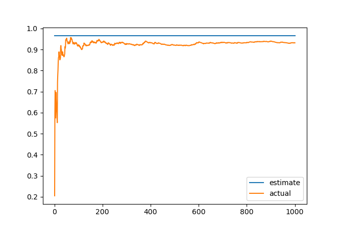
The real deal is comparing the variance of the estimated value with our formulas. I'm using the standard unbiased sample variance estimator to compute the variance from a number of observations, and compare it to the single-sample error predicted by the exact formula we've derived, for the uniform distribution:
and for the quadratic one:
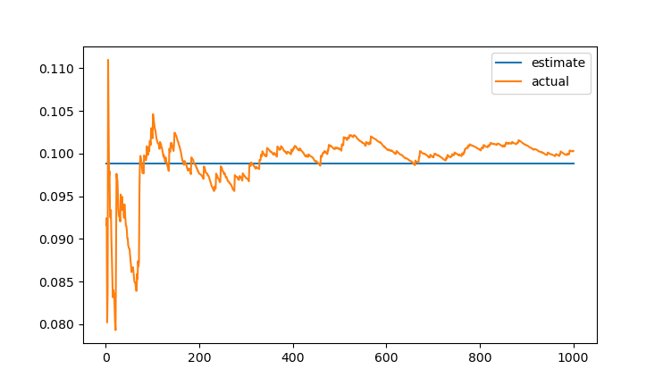
As expected, the observed error converges to the predicted one, with the quadratic distribution giving an order of magnitude smaller error. Hurray!
Specifically, after 1000 samples I got this values:
- The predicted single-sample error for uniform distribution is: 0.9668499904773105
- The observed single-sample error for uniform distribution is: 0.9707962784775023
- The predicted single-sample error for quadratic distribution is: 0.09888969900733573
- The observed single-sample error for quadratic distribution is: 0.10036578889793105
Not bad! This is just a single run, though; different runs produce different random results. You can try it yourself — the python script for generating these plots is available in this blog's repository.
Discussion
The first, approximate, formula for the variance is rather straightforward: the closer you are to the ideal distribution, the smaller the noise. The second, exact, formula is a bit more tricky.
We still get roughly the same behaviour thanks to the \(\varepsilon(x)^2\) in the numerator; however, there's a \(1+\varepsilon(x)\) term in the denominator.
If we overshoot the ideal probability, meaning \(p(x)>p^*(x)\) and thus \(\varepsilon(x)>0\), we have \(1+\varepsilon(x)>1\), and thus the error is even smaller than \(\varepsilon(x)^2\), which is nice!
If we undershoot, so that \(p(x)< p^*(x)\) and \(\varepsilon(x) < 0\), we have \(1+\varepsilon(x)<1\), making the error actually larger than \(\varepsilon(x)^2\).
It may seem that the answer is simple: just always try to overshoot! However, remember that both \(p(x)\) and \(p^*(x)\) are probability densities, and their integral over the whole domain \(\Omega\) is equal to 1, which constraints the amount of wiggle we can have when choosing a distribution. If we overshoot somewhere, we have to undershoot somewhere else, otherwise the total integral would be greater than 1!
However, notice that the error is not actually just \(\frac{\varepsilon(x)^2}{1+\varepsilon(x)}\), but rather the integral of this value times the ideal distribution \(p^*(x)\). Thus, the values of \(\varepsilon(x)\) matter more in areas where \(p^*(x)\) is large, i.e. where \(f(x)\) is large.
So, the general guideline seems to be to overshoot where \(f(x)\) is larger and undershoot where it's smaller. In other words, overfitting our distribution to areas where \(f(x)\) is large seems to be better than underfitting in these areas.
These claims seem to demand deriving their own numerical estimates, though...
Update: Philip Trettner noticed that this might explain why strong light sources produce fireflies when using e.g. cosine-hemisphere sampling as \(p(x)\): in this case \(p^*(x)\) is orders of magnitude larger than \(p(x)\) in the direction pointing to the light source, so \(\frac{p(x)}{p^*(x)} = 1+\varepsilon(x)\) is close to zero, thus \(\varepsilon(x) \approx -1\), and \(\frac{\varepsilon(x)^2}{1+\varepsilon(x)} \approx \frac{1}{1+\varepsilon(x)}\) where \(1+\varepsilon(x)\) is something close to zero, so the whole error value is extremely large. This is especially noticeable at grazing angles, where the cosine hemisphere distribution \(p(x)\) is even closer to zero, making \(1+\varepsilon(x)\) even closer to zero as well.