If you don't want a long an boring introduction, skip directly to the virtual pipes method description.
I will get a little bit sad if you do this, though x)
I'm somewhat obsessed with terrain generation, grid-based games, simulations, and stuff like that. And this stuff often involves water, — or at least it seems natural for water to be there.
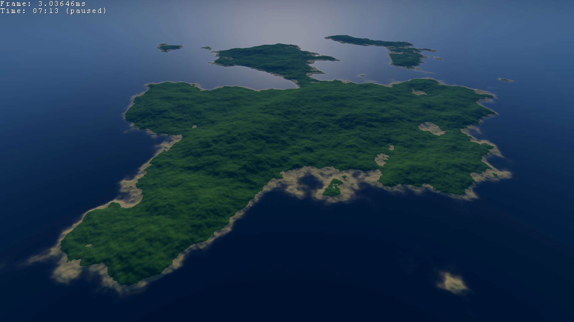
Say, you're generating a map for a strategy game, and you don't want the map borders to just be filled with inpenetrable void (like in old-school RTS games). Wouldn't it be nice for the border to be filled with water, like in this map from one of my abandoned projects:

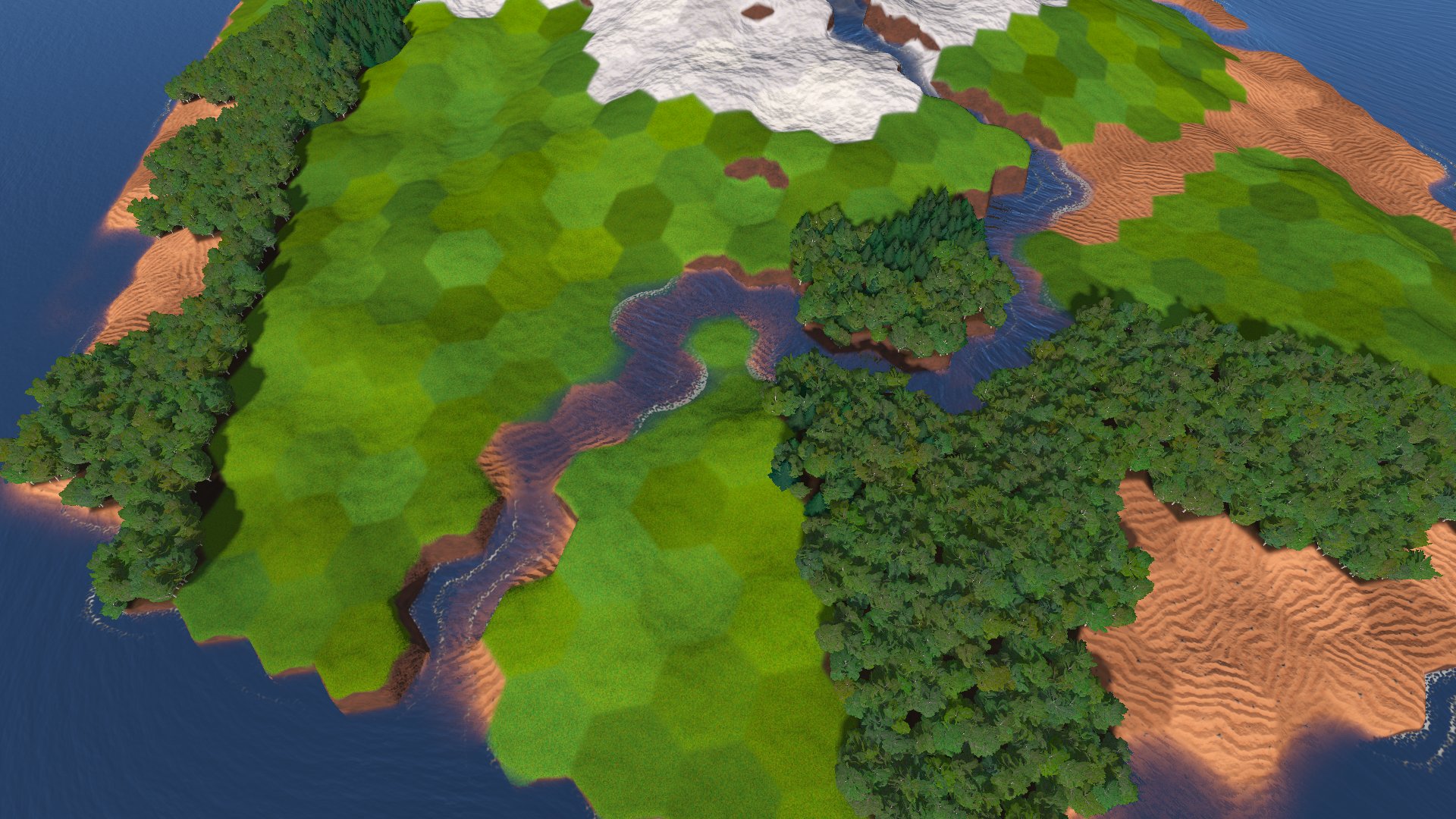
This provides a nice natural border, and maybe allows you to introduce some more water-related mechanics like sailing, fishing, trading, and sea warfare. Here's a 3D view of a similar island from the same project, for no particular purpose:
Or, say, you're making a peaceful village/town simulation game and you want your town to have a river for drinking, fishing, transportation, or even pure aesthetics. Or maybe you want a river just as a divider between areas, like in my first released game:
I hope I've convinved you: having water is really nice. (Not that it wasn't obvious anyway).
But water has problems.
Contents
Problems with water
Most games don't allow terrain modification, which is reasonable — not every game needs it. Even those that do can often get away with some simplistic approach: I can easily imagine being able to fill up a hill in a game like Civilization (though it would probably break a lot of stuff gameplay-wise), and it doesn't interact with water in any way.
My game, however, does need terrain modification:
Why? Well, uhm, because my design docs say so! I promise, it was somewhere on that page... or that one...
Seriously, though, there are indeed a couple of reasons in my case:
- Some resourses in my game are literally taken from the ground, like dirt, sand, and clay, and it just makes sense that when you dig them up, the ground gets removed (otherwise we'd get an infinite source, which is not ideal)
- Similarly, for stuff like stones & metal ores I'd prefer for them to get excavated from the ground when mining (instead of having a shiny "gold ore" boulder lying on the ground, as many games do), and it makes sense that the mined ground gets removed as well
- My game doesn't allow constructing buildings on slopes, so it's important to be able to level the terrain before building something on it, like in The Sims
- I want to give the player a ton of tools for creative expression, and terrain modification is one of them
- Let's be honest, everybody loves terrain modification
So, OK, that does this have to do with water? Say, you have a lake, or even a puddle, and you've dug up its border and opened a free passage for the water to flow out. What does the water do?
There are a number of simple options:
- Water doesn't go anywhere, and stays where it was initially generated (of course, this just feels boring and dumb)
- Water doesn't flow; instead, everything below a certain height level is considered water, like in Sapiens
- Water also exists below some level, but you can't even dig that far, or maybe you can only dig one level down to remove hills/mountains, like in RimWorld
- Water flows using some extremely simplistic model, like in Minecraft
- Water flows using some nice but still simplistic cellular-automata-ish model, like in Dwarf Fortress
Among these solutions, not one feels satisfactory to me. They are good fallbacks to consider if I fail to find a better option, but as a main water model they are just too...boring. Dwarf Fortress comes closer than others, but still, their model is too blocky yet also designed for 3D, which I don't really need (see the next section).
For years (yep, literally) I was passively searching for a model that would work for my needs. I researched a ton of literature on fluid simulations, particularly in climate & oceans/rivers simulations, and got really scared because most of the models used there are insanely complicated, while their applicability to my case was always blurry since the scientific community usually doesn't cover game design. One time I even managed to compute something like the expected currents flowing around an island, by solving a mass conservation equation for the liquid flow, i.e. something like \(\nabla (\text{mass}\cdot\text{velocity})=0\):
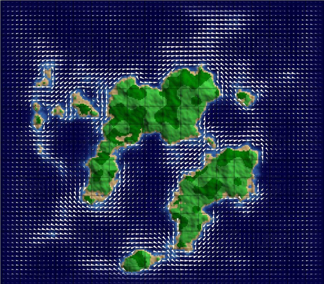
It's already something, but I need a dynamic model, not a static assignment of currents. (It can still be useful for some funny climate map generation, I guess.) By the way, it is theoretically easy to turn a dynamic model into a static one: just add equations like \(\frac{dX}{dt}=0\) for all your state variables \(X\), saying that you have a steady state (i.e. a solution that's perfectly stable and doesn't change with time, like a slowly flowing river).
I could just give up, of course. After all, it's important to remember that, in the end, I'm not making some reality simulator, — I'm making a game, and I'm free to bend the rules of it any way I see fit. However, I also couldn't shake off the feeling that some clever combination of simple formulas should work for my case. And I was right!
By the way, if reading this section made you scream "TIMBERBOOOORN" seven times, guess what: they use exactly the same model as I'm going to describe.
Also, if you know other models that you think would suit my case — tell me! I'd love to hear about them!
The setup
I've said the phrase "my case" four times already, but what exactly do I mean? Here's the list of features I want my water simulation to have:
- The simulation should probably work on a grid, preferably on the same grid I'm using for the terrain
- The average scale of the simulation should be around 1 meter or so, — I don't care about tiny splashes of water, while a kilometer-wide simulation is too coarse for something like a city builder game (I can easily add fake higher-frequency visual details on the rendering side without having to simulate them)
- I'm fine with assuming that water is a height field over the terrain, i.e. it doesn't flow vertically and it doesn't have gaps in vertical cross-sections, because my game's terrain is itself a height field, and because this basically reduces the problem to 2D
- Water should be able to flow (duh)
- Water shouldn't magically disappear due to simulation errors (this happens with some models I tried before)
- The simulation should be controllably stable
- The simulation should be fast enough, ideally the cost of a single simulation step should be linear in the simulation size (i.e. a few for-loops over the simulation domain)
As you can guess, I've found such a model, and this is what this article is about. But first,
Non-solutions
Let me describe a couple of popular options that do not suit my scenario.
Smoothed Particle Hydrodynamics is an insanely popular way to do fluid simulations which produces impressive results. However, this method also solves a completely different problem! It gives you realistic, highly detailed and beautiful simulations, which is not what I want. Remember the "average scale" thing I said earlier? Having 1 meter-sized water particles doesn't really work, — they'll look like water-filled balloons, — but having smaller particles hits performance too much. I don't need a high-detailed simulation, I want a fast and reasonable one!
Jos Stam's Stable Fluids is probably the most well-known fluid simulation work known in computer graphics, which also solves a different problem. It works with a full volume of fluid, rather than with a free surface like I need. Think of a closed tank filled with water, as opposed to water over terrain. It is also far from fast: some steps of the simulation require iteratively solving a sparse linear system, which is doable but still expensive.
In fact, I've implemented Stable Fluids once, and it's a really fun and impressive model, it's just a model for a different thing (it solves the full Navier-Stokes instead of the shallow water equations that we actually need):
Shallow water equations
Beware: I'm not a physicist, and this section might be full of complete nonsense.
Now, whenever we talk about seeking a mathematical model of something, it usually means we need some equations to solve. Generally, fluid motion is described by the Navier-Stokes equations, or by the simpler Euler equations. However, these equations also don't talk about a free water surface, but instead about a volume completely filled with fluid.
If we look at the variables these equations work with, we see fluid velocity, pressure, density, thermodynamic work, stress tensor, and some other things, and you'd need a good full course in fluid dynamics to figure out which of these are known, which are unknowns, and which can be derived from others (after lazily researching this for years I still don't know the answer, btw). Notice that there's nothing like "amount of water" here. We do have mass density, but all equations divide by it, so we can't really have zero density or a boundary between fluid and air. (This can actually be done using stuff like the particle-in-cell and marker-and-cell methods, if I'm not mistaken.)
Even in the simplest form, these equations involve pressure \(p\), which is unknown and changes with time, but there's no equation for how exactly it evolves! I.e. there's no \(\frac{dp}{dt}=\dots\) equation. Instead, the time evolution of the pressure field is implicitly built into the other equtaions. This is closely related to the projection step in the Stable Fluids solver.
What we need is to take something like Navier-Stokes, assume that we have a layer of water on top of some terrain (commonly called the bed in this case), and do some sort of averaging out along the vertical direction, so that we're left with purely 2D equations describing how water moves. That's exactly what the shallow water equations are about!
The "shallow" part means that we assume the typical vertical size of a water column to be much smaller than our typical horizontal scales. This is usually more or less true in things like modelling climate or river floods: the water heights (say, meters or tens of meters for a river) is much smaller than horizontal distances we're interested in (kilometers).
These equations are what is typically used in a lot of "water over terrain" situations in science, and they are what we're going to solve as well. I won't put the equations themselves here — you can find them on wikipedia, and that's not what this post is about. Instead, I'll describe the solution method directly, and try to make some sense of it.
Staggered grids
One thing we need to talk about before describing the full solution is the grid. Usually when numerically solving differential equations, we discretize the simulation area into a grid (say, a grid of squares), and store the values of our field (velocity, pressure, stuff like that) per grid cell or per grid vertex.
For example, when solving the wave equation (which works better for sound waves and EM waves rather than water waves), we store the wave height u(i,j) and it's time derivative du(i,j) per each cell, and then the update code is
du(i,j) += (u(i+1,j)+u(i,j+1)+u(i-1,j)+u(i,j-1)-4*u(i,j)) * dt/dx/dx;
u(i,j) += du(i,j) * dt;
It may be a bit cryptic, but the main idea is that both quantities are stored on the same grid. This leads to nice finite-difference equations, is simple to code, and generally makes sense.
Such grids are called collocated, which I always read as co-located: both quantities are located on the same grid. And such grids suck for fluid dynamics!
One reason is that they make finite difference methods confusing. In the wave equation we have the second derivative, which can be computed in a nice and symmetric way as
(f(x+1) + f(x-1) - 2*f(x)) / (dx * dx)But fluid dynamics feature first derivatives, in stuff like "the acceleration of fluid is proportional to the difference between how much water is on the left and the right". So, how do you compute this with finite differencies? (f(x+1) - f(x)) / dx makes the simulation biased to the right, may ignore some directional effects, and generally leads to instabilities. (f(x) - f(x-1)) / dx has the same problems. (f(x+1) - f(x-1)) / (2*dx) is nicely symmetric but ignores the value at the current cell f(x), which also leads to instabilities. In general, naive discretization of fluid dynamics equations is typically extremely unstable, and everything just oscillates in a stupid way instead of solving the equation.
Another way to see that this grid is not ideal is to consider this situation: assume that we store the water height and the water velocity vector in each cell. Now consider a cell that has incoming water flows both from left and right, and the water flows out to top and bottom cells. Here's an illustration:

The total velocity in this cell is zero! This is nonsense, since the water is clearly flowing quite a lot here.
Things like these led people to reconsider their grid methods, and invent something called staggered grids. There are many variants of these, but the typical one used for fluid simulation works like this: we store, say, water height/density/etc in square cells, but we store the velocity in edges between cells. Vertical edges (i.e. edges between horizontal neighbours) store the horizontal velocity, and vice versa. Here's an image:
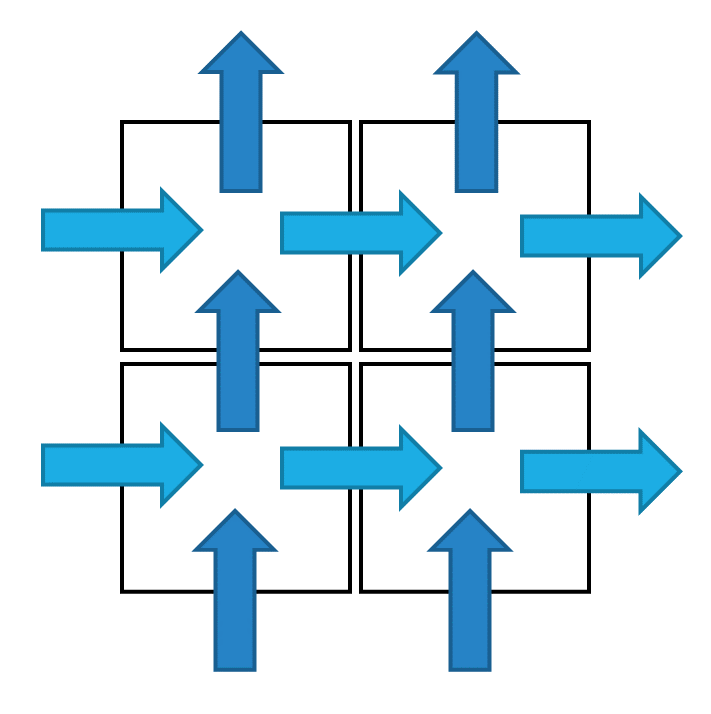
Blue arrows indicate the stored values, one per each edge between cells. Notice that the boundary edges are also here: these correspond to the boundary conditions of your simulation (we'll get to these a bit later).
So, if we want an \(N\times N\) square grid as our simulation area, we'd have to store
- \(N\times N\) array for, say, water height
- \((N+1)\times N\) array for X velocity
- \(N\times (N+1)\) array for Y velocity
This might feel unusual, but the sooner you accept it, the better your fluid simulations will get :)
Virtual pipes method
At last, we've arrived to the actual method I'm using for simulating water over terrain. This method is called virtual pipes, because it is derived by assuming that the water cells are connected by imaginary pipes of some radius. I used these two papers as a reference for this method. Notice that the first paper also consideres multi-level water columns and vertical connections, while the second paper is primarily about hydraulic erosion; I didn't really do any of these since that's not my goal.
First, for simplicity sake, let's ignore the terrain part, it will be trivial to add later. We'll store, just like in the previous section, three values on a staggered grid:
- \(N\times N\)
waterarray for the height of water surface in this cell - \((N+1)\times N\)
flowXarray for the total water flow between horizontally adjacent cells - \(N\times (N+1)\)
flowYarray for the total water flow between vertically adjacent cells
flowX(i,j) is the horizontal flow (also calles flux) between cells water(i-1,j) and water(i,j), unless it is a boundary edge (i == 0 or i == N), and similarly for flowY.
By the way, in what follows I'll use the notation array(i,j) to mean the i,j-th element of an array. In my actual C++ code the 2D arrays have an overloaded operator() to provide read-write element access, since multi-dimensional operator[] is only available since C++23.
Notice how we'll store the flow, not the velocity. To make sense of a flow, imagine you've put a magic curtain between two adjacent cells which can measure how much water goes through it. The water stream going through this curtain has a certain cross-section area, and it moves with some velocity. If you multiply this two values, you get water volume per unit of time, which is exactly what we'll store.
Flow tends to behave better than velocity when you have no water. For two adjacent empty cells, the flow between them is obviously zero, since there's no water to move. However, velocity is something like flow divided by water cross-section, i.e. zero divided by zero, which is always a problematic thing. You could say that in this case the velocity is obviously zero, but it's more subtle than that: what if both the water and the flow are very small, but non-zero? We'd quickly get into the territory of floating-point problems and discontinuities, and we'd have to figure out some thresholds such that below this water level threshold velocity is considered zero. All this is really messy, and working with flows instead of velocities just solves all these issues elegantly.
Enough talking, here are the three steps involved in the method:
Let's work them through one by one.
Flow acceleration
If you have two neighbouring water cells, and their water heights is different, basic reasoning tells us that water will flow from the larger to the smaller column. That's exactly what flow acceleration does: we take all interior (i.e. non-boundary) edges, and accelerate the flow in them based on the difference in water levels in corresponding water cells. We do this for the X flows:
for (int y = 0; y < N; ++y)
    for (int x = 1; x < N; ++x)
        flowX(x,y) += (water(x-1,y) - water(x,y)) * g * dt * A / dx;
and similarly for Y:
for (int y = 1; y < N; ++y)
    for (int x = 0; x < N; ++x)
        flowY(x,y) += (water(x,y-1) - water(x,y)) * g * dt * A / dy;
Here, dx and dy are the horizontal and vertical sizes of our cells (the lengths of the corresponding "pipes"), dt is the simulation time step (I'll talk about it later), g is the gravity, and A is the cross-section area of the virtual pipe. The paper takes A=dx*dx, while I took A=1. In general, A and g are only used in this step, and always as a product, so for our simple needs we can just ignore A and pretend that it is merged with g.
Usually, we also add friction to this step. Friction simply scales down the flow on each iteration, typically making the simulation converge to a static stable state. The paper recommends using a factor of pow(friction,dt) to make it dt-independent (which is closely related to exponential smoothing I've explained in another article). Thus, the simulation code becomes
for (int y = 0; y < N; ++y)
    for (int x = 1; x < N; ++x)
        flowX(x,y) = flowX(x,y) * pow(friction,dt)
                   + (water(x-1,y) - water(x,y)) * g * dt / dx;
and similarly for Y:
for (int y = 1; y < N; ++y)
    for (int x = 0; x < N; ++x)
        flowY(x,y) = flowY(x,y) * pow(friction,dt)
                   + (water(x,y-1) - water(x,y)) * g * dt / dy;
friction is typically between 0 and 1. friction=0 means maximal friction, i.e. the flow from the previous simulation step is completely annihilated. friction=1 means no friction at all. Because of this I'm actually using the formula pow(1-friction,dt) to make the friction value more intuitive. Of course, we should precompute the friction factor pow(1-friction, dt) at the start of simulation step, instead of computing it for each cell.
The time step dt is a bit tricky. Obviously, the larger it is, the faster the simulation goes. However, large values of dt also lead to instabilities. In general, there is a famous Courant-Friedrichs-Lewy condition (CFL) common to all fluid simulations. It states that, roughly speaking, the quotient dx/dt must not be less than the maximum speed of the fluid. In practice that means that we have to decrease dt (thus increasing the value of dx/dt) until the simulation becomes stable. I've used values around 0.001 and 0.01.
So, this step essentially acelerates the water flow, kinda like \(\frac{dv}{dt} = a = \frac{F}{m}\) from Newton's laws.
Water column updating
Yep, we'll first look at the third step of the simulation, because it will be important for understanding the second step.
This step is probably the simplest. For each water cell, we simply add or remove water according to the horizontal and vertical flows adjacent to this cell:
for (int y = 0; y < N; ++y)
    for (int x = 0; x < N; ++x)
        water(x,y) += (
                  flowX(x,  y) + flowY(x,y  )
                - flowX(x+1,y) - flowY(x,y+1)
            ) * dt/dx/dy;
flowX(x,y) and flowY(x,y) flow towards our water(x,y) cell, so we add them. The flows flowX(x+1,y) and flowY(x,y+1) flow out of our cell, thus we subtract them.
This step just moves the water between the cells, according to the computed flows. The \(\frac{dx}{dt} = v\) part of Newton's laws, if you like.
Outflow scaling
This second step is probably the trickiest. See, we might have a problem on step 3: if the outgoing flow is large enough, the amount of water in a cell can become negative! This is bad, since there's no such thing as a negative amount of water (as opposed to e.g. EM waves).
Fortunately, there is a simple solution called outflow scaling. We look at the flows adjacent to some water cell, and only consider the outgoing flows, i.e. flows that remove water from this cell, not add water. We take the total outgoing flow by summing these flows, and compare it to the actual amount of water in this cell. If we figure out that on the 3rd step we'll try to remove more water than the cell actually has, we simply scale the outgoing flows down, so that the water amount stays positive (or zero). Here's the code:
for (int y = 0; y < N; ++y) {
    for (int x = 0; x < N; ++x) {
        float total_outflow = 0.f;
        total_outflow += max(0.f, -flowX(x,y));
        total_outflow += max(0.f, -flowY(x,y));
        total_outflow += max(0.f, flowX(x+1,y));
        total_outflow += max(0.f, flowY(x,y+1));

        float max_outflow = water(x, y) * dx*dy/dt;

        if (total_outflow > 0.f) {
            float scale = min(1.f, max_outflow / total_outflow);

            if (flowX(x,y) < 0.f) flowX(x,y) *= scale;
            if (flowY(x,y) < 0.f) flowY(x,y) *= scale;
            if (flowX(x+1,y) > 0.f) flowX(x+1,y) *= scale;
            if (flowY(x,y+1) > 0.f) flowY(x,y+1) *= scale;
        }
    }
}
It's a bit messy due to having to filter only outgoing flows, but it gets the job done.
Terrain elevation
Now, we want water moving over terrain, but where's the terrain in these equations? Adding terrain is actually extremely easy. Imagine two neighbouring water cells with equal water column heights: they don't try to move into each other, because the water level is the same. Now let's imagine that the left cell has some non-zero terrain elevation below it. This moves the water surface height up, and now this cell's surface is higher than the right cell, and the water starts to move.
That is to say, when accelerating the flows, we simply need to replace the water column height by the water surface height, which is just terrain height plus column height.
If terrain(x,y) is the terrain elevation at a cell, then all we need is to update acceleration computations:
for (int y = 0; y < N; ++y)
    for (int x = 1; x < N; ++x)
        flowX(x,y) = flowX(x,y) * pow(friction,dt)
                   + (
                      water(x-1,y) + terrain(x-1,y)
                    - water(x,y) - terrain(x,y)
                   ) * g * dt / dx;
and similarly for Y:
for (int y = 1; y < N; ++y)
    for (int x = 0; x < N; ++x)
        flowY(x,y) = flowY(x,y) * pow(friction,dt)
                   + (
                      water(x,y-1) + terrain(x,y-1)
                    - water(x,y) - terrain(x,y)
                   ) * g * dt / dy;
Boundary conditions
When solving partial differential equations (which is what we're secretely doing here!), it's always important to consider what happens at the boundary of our simulation. For the virtual pipes method, the boundary conditions are implicitly defined by the boundary flow values, i.e.
- Left boundary:
flowX(0,y) - Right boundary:
flowX(N,y) - Bottom boundary:
flowY(x,0) - Top boundary:
flowY(N,0)
We can set these to whatever we want:
- Setting them to 0 makes them act like walls: water waves will simply collide with them
- Setting them to inflow (positive for left/bottom, negative for right/top) will make them add water to the simulation
- Setting them to outflow (negative for left/bottom, positive for right/top) will make them remove water from the simulation
For stuff like water over terrain, outflow boundary conditions seem reasonable (water on the edge of the map will simply disappear through the edge). If some parts of the boundary cross a river, we'd probably want this parts to be an inflow instead, so that the river actually, y'know, has flowing water in it.
It is important to set these values at the start of each simulation step, because outflow scaling can change them (and your outflow boundary can turn into a wall boundary).
Viscosity
The paper also adds viscosity to the simulation, simply scaling the flows by some factor that depends on the water height (thus, it is different from friction). The idea is that smaller water layers have trouble moving around due to various internal forces, but larger water layers can move freely. This turns into simply multiplying the flows by \(\frac{H^2}{H^2+3\cdot \Delta t\cdot \nu}\), where \(H\) is the water level of the cell where the flow originates (e.g. left cell for positive X-flow, and right cell for a negative X-flow), and \(\nu\) is the viscosity constant.
Here's the code:
for (int y = 0; y < N; ++y) {
    for (int x = 1; x < N; ++x) {
        float H = (flowX(x,y) > 0.f) ? water(x-1,y) : water(x,y);
        H *= H;

        if (H > 0.f)
            flowX(x,y) *= H/(H + 3*dt*viscosity);
    }
}
And similarly for Y:
for (int y = 1; y < N; ++y) {
    for (int x = 0; x < N; ++x) {
        float H = (flowY(x,y) > 0.f) ? water(x,y-1) : water(x,y);
        H *= H;

        if (H > 0.f)
            flowY(x,y) *= H/(H + 3*dt*viscosity);
    }
}
I imagine this could be useful for something like magma flow, but I didn't use it for water. The effects of viscosity are important on small scales (the paper applies it to blood flow inside organs), but on large terrain scales viscosity has almost no effect.
Full simulation code
So, here's the full simulation code that I used:
// Init boundary flows
for (int i = 0; i < N; ++i) {
    flowX(0,i) = ...; // left boundary
    flowX(N,i) = ...; // right boundary
    flowY(i,0) = ...; // bottom boundary
    flowY(i,N) = ...; // top boundary
}

// Precompute the friction factor
float frictionFactor = pow(1-friction,dt);

// Accelerate X-flows
for (int y = 0; y < N; ++y)
    for (int x = 1; x < N; ++x)
        flowX(x,y) = flowX(x,y) * frictionFactor
                   + (
                      water(x-1,y) + terrain(x-1,y)
                    - water(x,y) - terrain(x,y)
                   ) * g * dt / dx;

// Accelerate Y-flows
for (int y = 1; y < N; ++y)
    for (int x = 0; x < N; ++x)
        flowY(x,y) = flowY(x,y) * frictionFactor
                   + (
                      water(x,y-1) + terrain(x,y-1)
                    - water(x,y) - terrain(x,y)
                   ) * g * dt / dy;

// Scale outflows to prevent negative water amounts
for (int y = 0; y < N; ++y) {
    for (int x = 0; x < N; ++x) {
        float total_outflow = 0.f;
        total_outflow += max(0.f, -flowX(x,y));
        total_outflow += max(0.f, -flowY(x,y));
        total_outflow += max(0.f, flowX(x+1,y));
        total_outflow += max(0.f, flowY(x,y+1));

        float max_outflow = water(x, y) * dx*dy/dt;

        if (total_outflow > 0.f) {
            float scale = min(1.f, max_outflow / total_outflow);

            if (flowX(x,y) < 0.f) flowX(x,y) *= scale;
            if (flowY(x,y) < 0.f) flowX(x,y) *= scale;
            if (flowX(x+1,y) > 0.f) flowX(x+1,y) *= scale;
            if (flowX(x,y+1) > 0.f) flowX(x,y+1) *= scale;
        }
    }
}

// Update water columns
for (int y = 0; y < N; ++y)
    for (int x = 0; x < N; ++x)
        water(x,y) += (
                  flowX(x,  y) + flowY(x,y  )
                - flowX(x+1,y) - flowY(x,y+1)
            ) * dt/dx/dy;
And that's it! It might look intimidating at first, but as I've tried to explain earlier each step is actually pretty reasonable and intuitive. In the end, the bulk of the simulation is just 4 for-loops over a few 2D arrays with some fairly simple formulas inside.
You can have a look at full C++ update code here, though there's quite a bit of other stuff going on.
Here's what it looks like:
(The particles in the video are for visualization only, they don't take part in the simulation itself.)
Once you've found good parameter values (for dt and g), this thing seems to be stable as heck, while still satisfying all my requirements and generally looking more or less like water. Hooray!
Model shortcomings
Of course, this model isn't perfect. One of the most obvious problems is that it doesn't have inertia and velocity diffusion. A fast water stream entering a lake won't propagate further inside the lake, but will instead spread out in all directions, ignoring all accumulated inertia. Two parallel water streams going in opposite directions can exist and not interact with each other (provided the water levels are equal).
It also tends to create these waves when the water first enters some area, which looks a bit weird, but I guess this is acceptable:
Bonus: hex/triangular grids
My game actually uses a regular triangular grid, not a square one, because...reasons. In fact, Boris The Brave has neatly summarized all the advantages of such grids, and I'll refer you to his article.
Triangle grids can be seen as duals to hexagonal grids: just connect the centers of adjacent hexagons with lines, and they'll form a regular triangular grid. If we look at Red Blob Games' amazing article on hexagonal grids, what I'm using is basically the axial coordinate system on a dual to a pointy-top hex orientation.
What's cool is that we can store such grid in usual 2D arrays (just skewed a bit), and refer to vertices of such grid using X,Y coordinates:
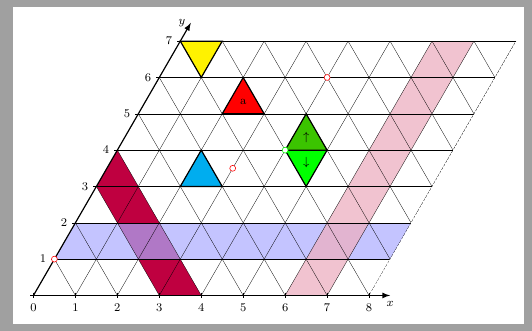
So, to simulate water on such a grid, I'll store water column height at grid vertices, which will make it easy to render the water surface (it's just a triangulation, much like the terrain itself).
The flows are a bit more complicated. There are flows in the X direction, flows in the Y direction, and flows in the...Z direction? Let's call it like that. Here's an illustration:
So, for each vertex, there are:
- X-flow coming from the left
- X-flow going to the right
- Y-flow coming from bottom-left
- Y-flow going to top-right
- Z-flow coming from bottom-right
- Z-flow going to top-left
For an \(N\times N\) grid of vertices, we have:
- \((N+1)\times N\) array of X-flows
- \(N\times (N+1)\) array of Y-flows
- \((N+1)\times (N+1)\) array of Z-flows, with the bottom-left and top-right values being unused
This way,
flowX(x,y)is the flow from(x-1,y)to(x,y)flowY(x,y)is the flow from(x,y-1)to(x,y)flowZ(x,y)is the flow from(x,y-1)to(x-1,y)
Not much changes from the square grid case, we just need to incorporate the Z-flow into 1) boundary conditions, 2) acceleration, 3) outflow scaling, and 4) water updating. The hardest part here is not to mess up the indexing :)
You can find the C++ code for such a simulation here. It works pretty well, and is hopefully a bit more isotropic than the square grid case :)
I've yet to implement all this in my game, though, — there are many, many more important things to do. But I'm quite determined that my game will have at least some form of basic water simulation now, which sounds super exciting. Imagine digging trenches to automatically water large farms, or diverting a river so that it floods a nearby village? The possibilities are endless. And for now, thanks for reading.