If you don't care about the explanation and want a direct link to the simulation, here you go.
You might know that I'm a sucker for physics simulations, and particle simulations in particular. Usually I implement something based on conventional physics, but recently I've stumbled upon a funny non-physical model that can display...well, let's call it life-like behavior.
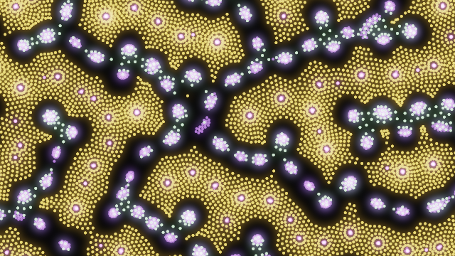
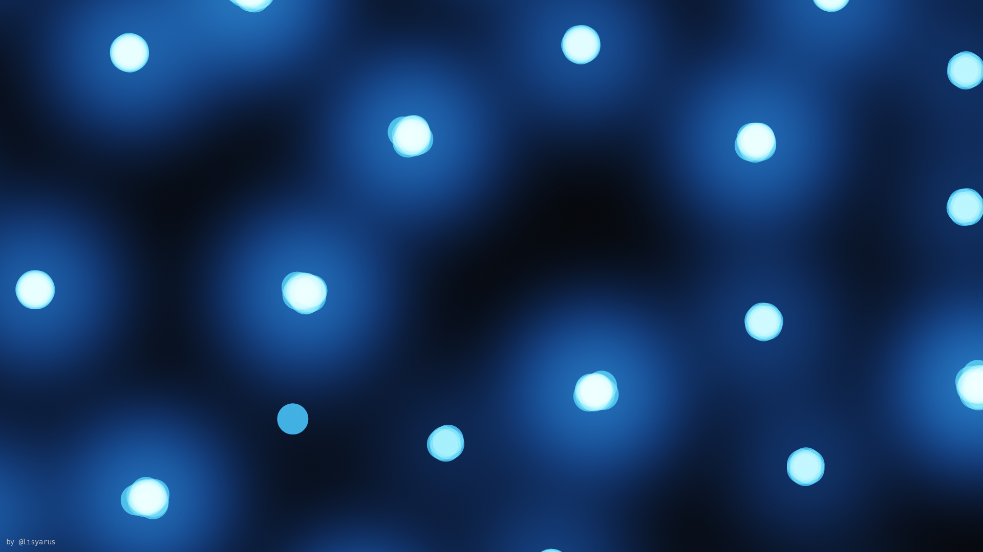
I've made a prototype in C++ using my pet engine, but then I decided it would be fun to try making it run in browser, using the WebGPU API. It works surprisingly well, and can produce fun simulations like this:
In this post I'll describe how it works under the hood.
Contents
The Particle Life Model
There are quite a number of resources (primarily, videos) online that talk about this model, for example this, this, and this, and also this one talks about the exact formulas used in the simulation. Due to a rather pretentious name composed of two overused words, googling "particle life" doesn't bring stuff of any relevance (apart from the YouTube videos), so I wasn't able to trace the origins of this model. One video claims that this model was inspired by some microbiology studies, which seems believable given how organic and mobile the resulting simulations look.
This model isn't in any way related to Conway's Game of Life (despite the name). It's more like Particle Lenia, if anything, though the rules are much simpler.
The core idea goes like this: we run a typical physics simulation with point particles, but the forces between particles can be asymmetric: particle A can attract particle B, but particle B can repel particle A (or attract it with a larger/smaller force, etc). This immediately violates Newton's third law, thus it violates almost all conservation laws (specifically, energy, momentum, and angular momentum conservation).
This might sound strange and unphysical, but
- We're not bound by physical laws when coding simulations,
- This brings an extra source of energy, which is kinda what living organisms do.
Living creatures consume food and oxygen (and sometimes other chemicals) and turn them into energy, which they can use to move and find more consumable stuff. The asymmetric forces of Particle Life emulate that by skipping the chemicals-to-energy cycle and just adds extra energy to the system.
It also allows particles to chase each other, e.g. in the scenario above particle B will constantly chase after particle A, which will in turn run away from particle B, which also kinda emulates predator-prey stuff from biology. However, in this model particles aren't created or destroyed, so particle B will never actually "eat" particle A.
For simplicity and to add some coherence to the simulation, particles are usually split into several types, with a table specifying the interaction for each pair of particle types. Specifically, I used the model suggested by this video:
- For any two particle types A and B, the force experienced by A from B consists of two parts: the interaction force, and the collision force.
- Interaction force can be either attractive or repulsive.
- Collision force is always repulsive.
- Both forces are specified by a radius and a strength factor. Positive strength means attraction, negative strength means repulsion. (For collision force it is always repulsion).
- Collision force radius is always smaller than interaction force radius (i.e. collision is close-range, interaction is far-range).
- Collision force strength is always larger than interaction force strength.
- Both forces decrease linearly with distance, upon reaching the radius value, at which they are zero.
In formulas, the linear dependence of force on distance can be written as
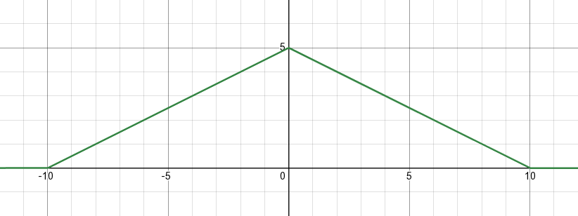
\[ F(r) = A\cdot \max\left(0, \frac{|r-R|}{R}\right) \]where \(A\) is the force strength (negative for repulsion), \(R\) is the force radius, and \(r\) is the distance between the two particles.
Here's a plot of force as a function of distance, with \(A=5\) and \(R=10\):
And here's the corresponding potential energy, if you're into some physics:

Here's the Desmos link where you can play with these values.
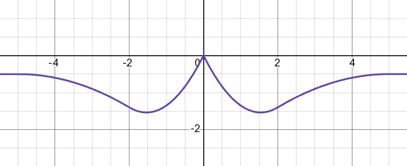
If we add the collision force and, say, an attraction force, we get this plot of force vs distance:
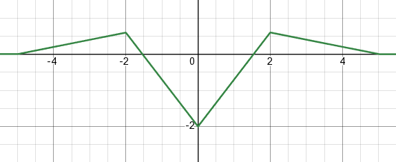
And the potential energy:
Again, here's the Desmos link for these.
As you can see, for the collision + attraction case, there's a local minimum at some distance, where the force is equal to zero. This would be the "sweet spot" for particles, i.e. they'll tend to maintain this distance if possible.
Notice that the force (and thus also the energy) doesn't go to infinity when distance is close to zero, like it does in a typical \(\frac{1}{r}\) potential from gravity or electromagnetism. This means that our collision force has finite strength, and can be overcome by sufficiently strong other forces, or if the collision radius is small enough. E.g. on this screenshot multiple particles merged into one:
This is fine, though, since it produces interesting behaviours, and it prevents our forces from escalating too much (which typically happens with a \(\frac{1}{r}\) potential simulations).
I also have a global constant friction parameter which simply decreases all velocities with time. This is to keep the simulation somewhat stable, because otherwise it constantly gains energy, and everything just accelerates to infinity.
Why WebGPU?
It should be clear why I decided to move the simulation to the GPU — after all, that's a typical massively parallel task, and GPUs shine at those. But why specifically WebGPU?
If you've been following me for a while, you might know that I'm in awe with WebGPU. I've been using OpenGL for more than a decade and I'm sick of it. It's a very old, stupidly inconsistent API full of legacy decisions, which stopped evolving some 8 years ago. However, Vulkan, which is the supposed alternative modern API, takes 1000 lines of setup work just to show a triangle on screen, without even any vertex buffers & attributes. Don't get me wrong, Vulkan is pretty cool, but I just don't have that much spare time to use it in my pet projects.
Now, WebGPU fills this niche for me. It is a modern & clean API that at the same time is reasonably non-verbose. It feels just like what real-time graphics should be about, — or at least that's what I feel while using it. I already used it in a few desktop projects (via wgpu-native), including a full Monte-Carlo raytracer and a shallow water simulator, and I'm using it in my current main project, which is a medieval village building game, and I'm really happy with this API.
Furthermore, being a modern API, it supports stuff like compute shaders and atomics, which are crucial for this simulation, as we'll see later. As far as I know, WebGL doesn't support these features.
And, as a nice bonus, it actually runs in browser! Or, at least in some experimental versions of some browsers, under some flags, but the situation should get better with time.
Simulation loop
So, how do we simulate particles with WebGPU? The simulation loop itself is rather straightforward:
- If not paused,
- For each particle, compute the forces acting on this particle by other particles, and add the resulting acceleration to the particle's velocity
- For each particle, move its position using the newly-computed velocity
- Apply boundary conditions
- Render the particles
This is essentially the semi-implicit Euler integrator, which is easy to code and has some nice theoretical properties.
I store the particles in a single large GPU buffer. A particle is just a simple struct like this:
struct Particle
{
    // Position
    x : f32,
    y : f32,

    // Velocity
    vx : f32,
    vy : f32,

    // Type
    species : f32,
}
I'm not storing position and velocity as vec2f just for alignment requirements, and I'm storing the particle type as an f32 just to be able to load particles from JavaScript as a single large Float32Array.
So, a particle is just 5 floats, i.e. 20 bytes. In theory, we could just run a single compute shader per particle, which loops over all particles, computes all the forces, and updates velocity and position. However, computing forces quickly becomes the bottleneck: it's a \(O(N^2)\) operation in total, because we need to compute all pairwise forces between all particles. This severely limits the number of particles we can process. My earlier CPU implementation only got to 4096 particles, even with multithreading.
We need to be clever about computing forces, which is why this is a separate compute pass. After that, things are pretty straightforward: a single compute shader invocation for each particle moves it forward using the computed velocity, then handles collisions with simulation borders:
@group(0) @binding(0) var<storage, read_write> particles : array<Particle>;

@group(1) @binding(0) var<uniform> simulationOptions : SimulationOptions;

@compute @workgroup_size(64)
fn particleAdvance(@builtin(global_invocation_id) id : vec3u)
{
    // Protect against reading & writing past array end
    if (id.x >= arrayLength(&particles)) {
        return;
    }

    let width = simulationOptions.right - simulationOptions.left;
    let height = simulationOptions.top - simulationOptions.bottom;

    var particle = particles[id.x];

    // Apply friction
    particle.vx *= simulationOptions.friction;
    particle.vy *= simulationOptions.friction;

    // Move particle using velocity
    particle.x += particle.vx * simulationOptions.dt;
    particle.y += particle.vy * simulationOptions.dt;

    // Collide with borders
    if (particle.x < simulationOptions.left) {
        particle.x = simulationOptions.left;
        particle.vx *= -1.0;
    }

    if (particle.x > simulationOptions.right) {
        particle.x = simulationOptions.right;
        particle.vx *= -1.0;
    }

    if (particle.y < simulationOptions.bottom) {
        particle.y = simulationOptions.bottom;
        particle.vy *= -1.0;
    }

    if (particle.y > simulationOptions.top) {
        particle.y = simulationOptions.top;
        particle.vy *= -1.0;
    }

    // Write the new state of the particle
    particles[id.x] = particle;
}
(My actual code also handles mouse interaction & looping borders, but the idea is the same.)
The simulationOptions.friction is actually something like \(\exp(-\text{friction}\cdot\Delta t)\), for reasons explained in my other article.
Computing interactions
Before advancing the particles, though, we need to compute the inter-particle forces. The main trick is to use the fact that all forces have finite radius, and after a certain distance all forces are zero. In my implementation, I only allow forces with radius up to 32. Thus, I know that any pair of particles further than 32 units of distance apart cannot interact at all.
To utilize this, we use the typical approach of spatial hashing/binning: make a square grid with cells/bins of size \(32\times 32\), sort the particles into these bins, then compute interactions only between neighbouring bins. This sounds easy, and is actually almost trivial to implement on the CPU (e.g. in C++ just make a 2D array, each storing std::vector<particle>, and you're good to go). However, building such data structures on the GPU takes a lot of effort — we can't, for example, allocate GPU memory directly from a shader!.
Instead, we'll use a linearized structure to store the bins. Here's how it works: we'll have an array of particles, where particles that reside in the same bin occupy a contiguous section of this array. Then, we'll also have an array which stores the start of this section (i.e. the offset) for each bin. We don't need to store the end of it, because the end of a bin is exactly the start of the next bin! We could also store the particle IDs instead of particles themselves, but that's another indirection which could hurt memory access performance later, when we compute the forces.
To do this, we use a typical three-phase approach:
- Phase 1: compute the number of particles in each bin
- Phase 2: run parallel prefix sum to compute the offset for each bin
- Phase 3: place each particle into the corresponding bin
Phases 1 and 3 make heavy use of shader atomics. Phase 1 is fairly simple — run a compute shader for each particle, compute the (linearized) bin index for this particle, and increment the size of this bin:
@group(0) @binding(0) var<storage, read> particles : array<Particle>;

@group(1) @binding(0) var<uniform> simulationOptions : SimulationOptions;

@group(2) @binding(0) var<storage, read_write> binSize : array<atomic<u32>>;

@compute @workgroup_size(64)
fn fillBinSize(@builtin(global_invocation_id) id : vec3u)
{
    if (id.x >= arrayLength(&particles)) {
        return;
    }

    // Read the particle data
    let particle = particles[id.x];

    // Compute the linearized bin index
    let binIndex = getBinInfo(vec2f(particle.x, particle.y),
        simulationOptions).binIndex;

    // Increment the size of the bin
    atomicAdd(&binSize[binIndex + 1], 1u);
}
Since this is done in parallel by many shader invocations, we need to use atomics here. I'm actually incrementing array at index binIndex + 1, and leaving the 0-th element at the value of 0, because this way binOffset[i + 1] - binOffset[i] always gives you the size of the i-th bin. Note that in this case the binSize array size is 1 plus the actual number of bins.
Here, getBinInfo is just some helper function that computes the linearized bin index from the particle position and the size of the whole grid of bins:
fn getBinInfo(position : vec2f, simulationOptions : SimulationOptions) -> BinInfo
{
    let binSize = simulationOptions.binSize;
    let gridSize = simulationOptions.gridSize;

    let binId = vec2i(
        clamp(i32(floor((position.x - simulationOptions.left) / binSize)), 0, gridSize.x - 1),
        clamp(i32(floor((position.y - simulationOptions.bottom) / binSize)), 0, gridSize.y - 1)
    );

    let binIndex = binId.y * gridSize.x + binId.x;

    return BinInfo(binId, binIndex);
}
(N.B.: in my actual code, gridSize is not passed as a uniform, but computed in-place, because I did it this way first and then never changed that.)
In Phase 2, we need to convert the array of bin sizes into an array of bin offsets. Since the particles from the same bin go continuously in memory, a bin with some index starts when we've already put all the particles from bins with smaller indices into the array. This means that the offset \(O[i]\) of the i-th bin is simply the sum of the sizes \(S[j]\) of all preceding bins: \(O[i] = \sum\limits_{j=0}^{i-1} S[j]\). In pseudocode:
offset[0] = 0;
for (int i = 1; i < binCount; ++i)
    binOffset[i] = binOffset[i - 1] + binSize[i];
This is known as computing prefix sums. This is, of course, not a parallel algorithm. To harness the power of the GPU, we'd want to run a parallel algorithm that does that. This is known, of course, as the parallel prefix sum problem, and we'll talk about it in the next section.
For now, let's assume we've computed these offsets somehow. In Phase 3, we need to place ("sort") the particles into a new array, based on which bin this particle belongs to. We do this by running a per-particle compute shader once again. Because we want to put different particles into different indices in the new array, we need to use atomics again:
@group(0) @binding(0) var<storage, read> source : array<Particle>;
@group(0) @binding(1) var<storage, read_write> destination : array<Particle>;
@group(0) @binding(2) var<storage, read> binOffset : array<u32>;
@group(0) @binding(3) var<storage, read_write> binSize : array<atomic<u32>>;

@group(1) @binding(0) var<uniform> simulationOptions : SimulationOptions;

@compute @workgroup_size(64)
fn sortParticles(@builtin(global_invocation_id) id : vec3u)
{
    if (id.x >= arrayLength(&source)) {
        return;
    }

    // Read the particle data
    let particle = particles[id.x];

    // Compute the linearized bin index
    let binIndex = getBinInfo(vec2f(particle.x, particle.y),
        simulationOptions).binIndex;

    // Atomically compute the index of this particle
    // within the corresponding bin
    let indexInBin = atomicAdd(&binSize[binIndex], 1);

    // Write the particle into the sorted array
    let newParticleIndex = binOffset[binIndex] + indexInBin;
    destination[newParticleIndex] = particle;
}
Here, we need to zero out the binSize array before running this shader. Again, since multiple shaders run in parallel, we use atomics to compute the index of a particle within its bin.
Once we've done that, we can easily iterate over particles of a specific bin, which allows us to run the actual shader that computes per-particle forces, by only iterating over the neighbouring bins. Once again, a single shader invocation per each particle:
@group(0) @binding(0) var<storage, read_write> particles : array<Particle>;
@group(0) @binding(1) var<storage, read> binOffset : array<u32>;
@group(0) @binding(2) var<storage, read> forces : array<Force>;

@group(1) @binding(0) var<uniform> simulationOptions : SimulationOptions;

@compute @workgroup_size(64)
fn computeForces(@builtin(global_invocation_id) id : vec3u)
{
    if (id.x >= arrayLength(&particles)) {
        return;
    }

    // Read particle data
    var particle = particles[id.x];
    let type = u32(particle.type);

    // Compute the bin that contains this particle
    let binInfo = getBinInfo(vec2f(particle.x, particle.y), simulationOptions);

    // Compute the range of neighbouring bins for iteration
    var binXMin = binInfo.binId.x - 1;
    var binYMin = binInfo.binId.y - 1;
    var binXMax = binInfo.binId.x + 1;
    var binYMax = binInfo.binId.y + 1;

    // Guard against grid boundaries
    binXMin = max(0, binXMin);
    binYMin = max(0, binYMin);
    binXMax = min(binInfo.gridSize.x - 1, binXMax);
    binYMax = min(binInfo.gridSize.y - 1, binYMax);

    let particlePosition = vec2f(particle.x, particle.y);

    var totalForce = vec2f(0.0, 0.0);

    // Iterate over neighbouring bins
    for (var binX = binXMin; binX <= binXMax; binX += 1) {
        for (var binY = binYMin; binY <= binYMax; binY += 1) {
            // Compute linearized bin index
            let binIndex = binY * binInfo.gridSize.x + binX;

            // Find the range of particles from this bin
            let binStart = binOffset[binIndex];
            let binEnd = binOffset[binIndex + 1];

            // Iterate over particles from this bin
            for (var j = binStart; j < binEnd; j += 1) {
                // Prevent self-interaction
                if (j == id.x) {
                    continue;
                }

                let other = particlesSource[j];
                let otherType = u32(other.type);

                // Apply the inter-particle force

                let force = forces[type * u32(simulationOptions.typeCount) + otherType];

                var r = vec2f(other.x, other.y) - particlePosition;
                let d = length(r);

                if (d > 0.0) {
                    let n = r / d;

                    totalForce += force.strength * max(0.0, 1.0 - d / force.radius) * n;
                    totalForce -= force.collisionStrength * max(0.0, 1.0 - d / force.collisionRadius) * n;
                }
            }
        }
    }

    // Update velocity, assuming unit mass
    particle.vx += totalForce.x * simulationOptions.dt;
    particle.vy += totalForce.y * simulationOptions.dt;

    particles[id.x] = particle;
}
(My actual code also includes a central force & handling looping boundaries. I also read particles from one buffer and write them to another buffer, but the idea is the same.)
forces is a \(M^2\)-sized array (where \(M\) is the number of particle types) which stores the inter-particle force parameters.
Parallel prefix sum
Computing prefix sums in parallel is a well-known problem. I'm using the simplest solution, outlined as the Algorithm 1 in the wikipedia article, and also called the naive parallel scan in this GPU Gems 3 article.
The image from wikipedia explains everything rather nicely:
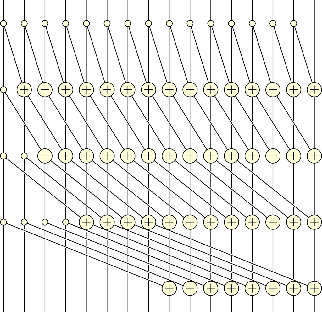
The main idea is to run several sweeps over the whole array \(\log_2(N)\) times (where \(N\) is the array size), each time adding x[i-step] to x[i], where step is a power of 2. In pseudocode, at iteration k we do
step = (1 << k);
parallel for (int i = step; i < array.size; ++i)
    array[i] += array[i - step];
We start iteration from i = step because otherwise at array[i - step] we'd try reading at an address before the array starts. This code won't actually work because overwriting array[i] affects what other invocations (with different values of i) will read, so we have to use 2 arrays: one for reading, and one for writing. Something like this:
parallel for (int i = 0; i < input.size; ++i) {
    if (i < step)
        output[i] = input[i];
    else
        output[i] = input[i] + input[i - step];
}
Then, to compute the actual prefix sum, we create a temporary array, and we ping-pong the input & temporary arrays \(\log_2(N)\) times with step taking the values of increasing powers of 2. On the first iteration (k = 0, step = 1), our binSize array is the input, and the temporary array is the output. On the next iteration (k = 1, step = 2), the temporary array is the input, and the binSize array is the output, and so on. In terms of WebGPU, this requires creating two bind groups with the same layout, one that reads from binSize array and writes to temporary array, and the other does the opposite.
Now, with this method, the resulting prefix sum will be in the first or the second array, depending on the parity of the number of steps performed, i.e. the parity of \(\log_2(N)\). That's rather inconvenient, so I always round it up to the closest even number: this way, the result is always in the same binSize array, while an extra prefix sum iteration would simply copy one buffer into the other automatically (look what happens with the code when step >= array.size).
That's a lot of talking, but the implementation is rather simple:
@group(0) @binding(0) var<storage, read> input : array<u32>;
@group(0) @binding(1) var<storage, read_write> output : array<u32>;
@group(0) @binding(2) var<uniform> stepSize : u32;

@compute @workgroup_size(64)
fn prefixSumStep(@builtin(global_invocation_id) id : vec3u)
{
    if (id.x >= arrayLength(&input)) {
        return;
    }

    if (id.x < stepSize) {
        output[id.x] = input[id.x];
    } else {
        output[id.x] = input[id.x - stepSize] + input[id.x];
    }
}
In order to supply different stepSize values while still keeping the whole thing as a single compute pass, I have a buffer with all stepSize values I need, and use it as the source for the uniform stepSize value with proper dynamic offsets in the GPUComputePassEncoder.setBindGroup call.
So, with \(\log_2(N)\) iterations (rounded up to an even number), we run this compute shader (one invocation per bin, — or, in my case, binCount + 1 invocations for reasons I outlined earlier), while ping-ponging two buffers. Here's what it looks like in JavaScript:
prefixSumIterations = Math.ceil(Math.ceil(Math.log2(binCount + 1)) / 2) * 2;

...

binningComputePass.setPipeline(binPrefixSumPipeline);
for (var i = 0; i < prefixSumIterations; ++i) {
    binningComputePass.setBindGroup(0, binPrefixSumBindGroup[i % 2], [i * 256]);
    binningComputePass.dispatchWorkgroups(Math.ceil((binCount + 1) / 64));
}
(The i * 256 dynamic offset is due to requirements that dynamic offsets must be a multiple of 256 bytes. The Math.ceil((binCount + 1) / 64) workgroup count is because the shader uses a workgroup size of 64, and I run it on an array of size binCount + 1.)
I could use a more sophisticated prefix sum algorithm, but there was no need to: even with e.g. 10000 bins, this whole particle sorting & prefix sum computation takes about 0.1ms on my GeForce GTX 1060. The whole performance is always dominated by inter-particle forces computation, so optimizing the binning step gives little profit.
Rendering
I render particles as squares which are transformed into perfect circles in the fragment shader. For each particle, I have 2 triangles, thus 6 or 4 vertices (with or without vertex duplication), all sharing the data of the same particle. That's rather inconvenient: I'd rather not duplicate the particle data and not use instancing for that. So, instead my vertices don't have any attributes, and instead read the particles array directly as a read-only storage buffer, based on the vertex ID:
@group(0) @binding(0) var<storage, read> particles : array<Particle>;
@group(0) @binding(1) var<storage, read> species : array<Species>;
@group(1) @binding(0) var<uniform> camera : Camera;

struct VertexOut
{
    @builtin(position) position : vec4f,
    @location(0) offset : vec2f,
    @location(1) color : vec4f,
}

const offsets = array<vec2f, 6>(
    vec2f(-1.0, -1.0),
    vec2f( 1.0, -1.0),
    vec2f(-1.0,  1.0),
    vec2f(-1.0,  1.0),
    vec2f( 1.0, -1.0),
    vec2f( 1.0,  1.0),
);

@vertex
fn vertexCircle(@builtin(vertex_index) id : u32) -> VertexOut
{
    let particle = particles[id / 6u];
    let offset = offsets[id % 6u] * 1.5;
    let position = vec2f(particle.x, particle.y) + offset;
    return VertexOut(
        vec4f((position - camera.center) / camera.extent, 0.0, 1.0),
        offset,
        species[u32(particle.species)].color
    );
}
Executed with a vertex count of 6 * particleCount, this produces a square per each particle. The fragment shader computes the distance in pixels from the fragment to the center of the particle, and turns it into the alpha value to produce a perfectly anti-aliased circle:
@fragment
fn fragmentCircle(in : VertexOut) -> @location(0) vec4f
{
let alpha = clamp(camera.pixelsPerUnit * (1.0 - length(in.offset)) + 0.5, 0.0, 1.0);
return in.color * vec4f(1.0, 1.0, 1.0, alpha);
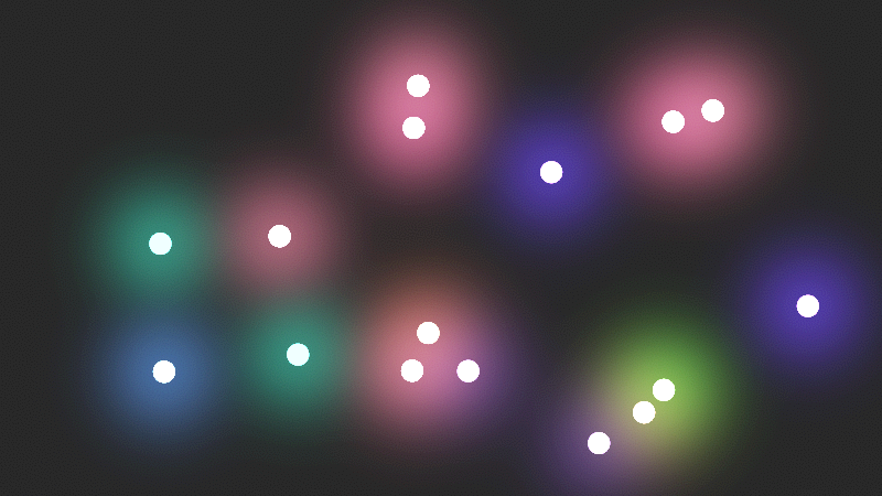
}And this is what it looks like:
I also add some glowing effect to the particles, which is rendered in a separate pass before the particles themselves. It works in pretty much the same way, but the squares are larger, and the alpha value is a gaussian:
@vertex
fn vertexGlow(@builtin(vertex_index) id : u32) -> VertexOut
{
    let particle = particles[id / 6u];
    let offset = offsets[id % 6u];
    let position = vec2f(particle.x, particle.y) + 12.0 * offset;
    return CircleVertexOut(
        vec4f((position - camera.center) / camera.extent, 0.0, 1.0),
        offset,
        species[u32(particle.species)].color
    );
}

@fragment
fn fragmentGlow(in : VertexOut) -> @location(0) vec4f
{
    let l = length(in.offset);
    let alpha = exp(- 6.0 * l * l) / 64.0;
    return in.color * vec4f(1.0, 1.0, 1.0, alpha);
}
All this is rendered using basic additive blending (not the usual over blending!) into an HDR rgba16float texture, then composited onto the screen (actually, onto an HTML canvas) using ACES tone-mapping and some blue-noise dithering to hide banding resulting from dark colors on the edge of the glow. I experimented with different blending methods & tone-mapping curves, and this combination produced the best visuals for my taste.
However, rendering perfect circles stops working when particles get too small, e.g. less than 1 pixel: the circle gets severely undersampled, the computed alpha values are pretty much random, and the whole image is just a big flickering mess. To counter that, I have a separate shader which replaces the circles when particle radius gets smaller than 1 pixel. It also renders squares, but the vertex shader makes sure the squares are exactly 2x2 pixels in size:
@vertex
fn vertexPoint(@builtin(vertex_index) id : u32) -> VertexOut
{
    let particle = particles[id / 6u];
    let offset = 2.0 * offsets[id % 6u] / camera.pixelsPerUnit;
    let position = vec2f(particle.x, particle.y) + offset;
    return CircleVertexOut(
        vec4f((position - camera.center) / camera.extent, 0.0, 1.0),
        offset,
        species[u32(particle.species)].color
    );
}
Then, the fragment shader computes the area of the intersection of the circle and the current pixel. Because computing circle-square intersections is a bit non-trivial, I approximate the circle with a square, compute the intersections (which boil down to min/max along each coordinate), and multiply by \(\frac{\pi}{4}\) to compensate for the square area vs circle area:
@fragment
fn fragmentPoint(in : CircleVertexOut) -> @location(0) vec4f
{
    let s = vec2f(camera.pixelsPerUnit);
    let d = max(vec2f(0.0), min(in.offset * s + 0.5, s) - max(in.offset * s - 0.5, - s));
    let alpha = (PI / 4.0) * d.x * d.y;
    return vec4f(in.color.rgb, in.color.a * alpha);
}
This feels hacky, but it works: the image almost doesn't flicker, and the transition between the two rendering modes is pretty much unnoticeable.
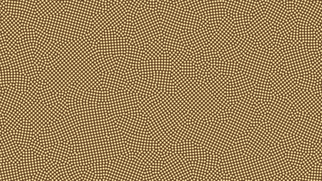
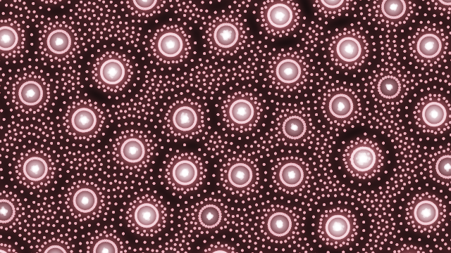
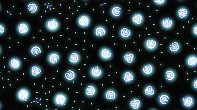
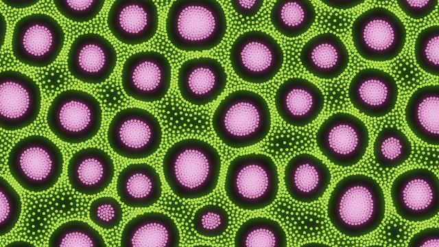
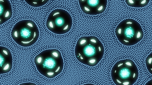
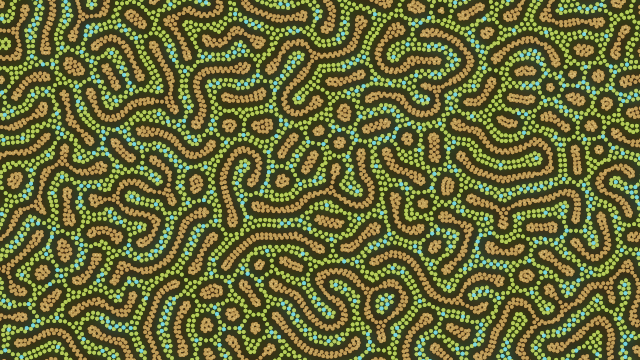
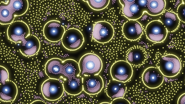
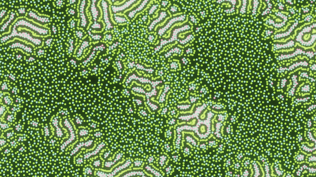
Gallery
I already posted the link in the beginning of the article, but if you don't feel like scolling back, here is the link to the simulation. Each page reload gives a new random system, though you can also just click "Randomize". You can save the current rules as a JSON file, or upload custom rules. You can share a randomly-generated rule set by clicking "Copy link".
I've noticed that less particle types leads to more large-scale coherent structures, while more particle types leads to more local & busy systems. Sometimes it is a good idea to do some simulated annealing and slowly increase or decrease the friction value, which works kind of like the inverse temperature here.
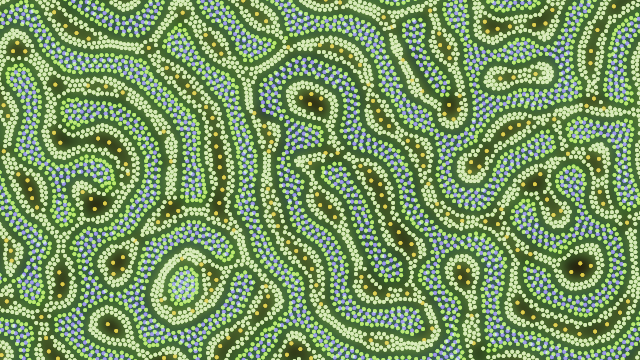
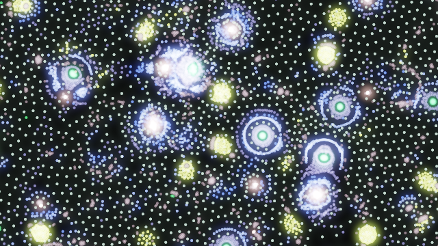
But, honestly, pretty much any random system made with this simulator looks interesting in some way. Here are some of the cool-looking systems I've been able to find in about 15 minutes. Each image is a link to this particular system: